CS180 Project 2

Part 1

This part of the project explores taking derivatives and gradient-magnitudes of images. One can observe the effects of blurring (low-pass filtering) an image on its derivatives and gradient magnitudes.

1.1

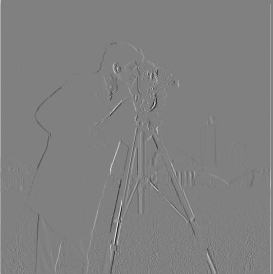
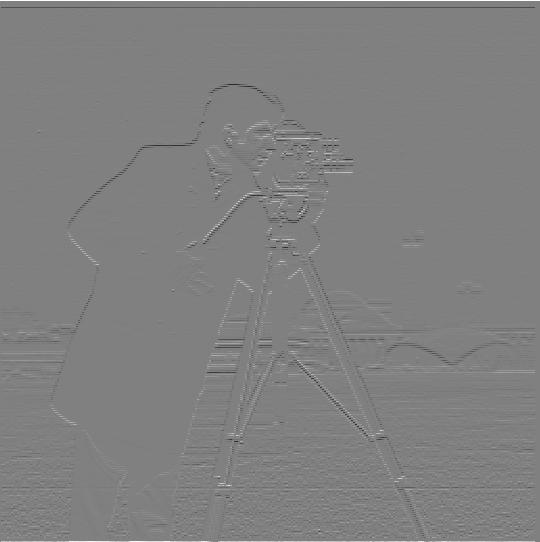
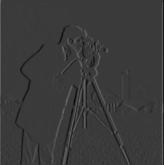
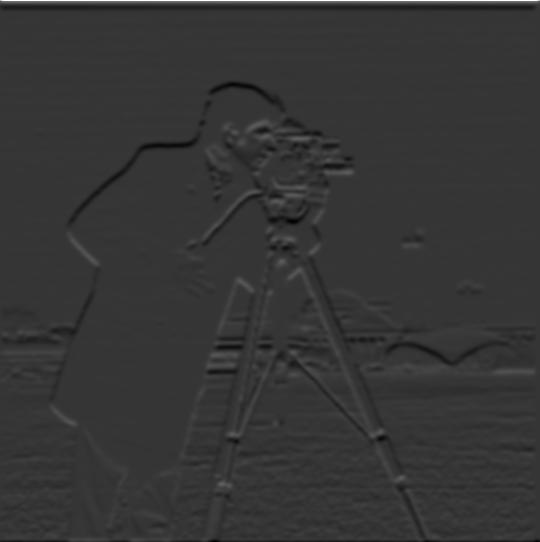
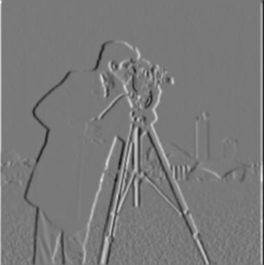
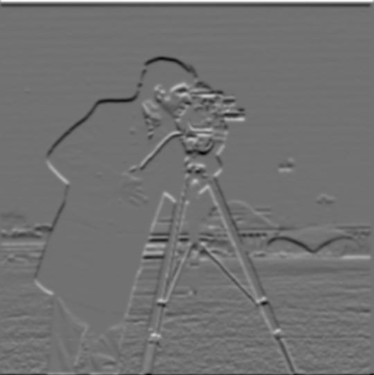
For the first part, I convolved the first channel of the input image (cameraman.png) with the finite difference operators. These convolutions simulate taking the derivative of the input image with respect to either x or y. The resulting images display where changes in value occur across the horizontal or vertical directions.

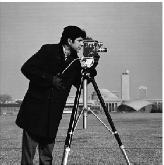
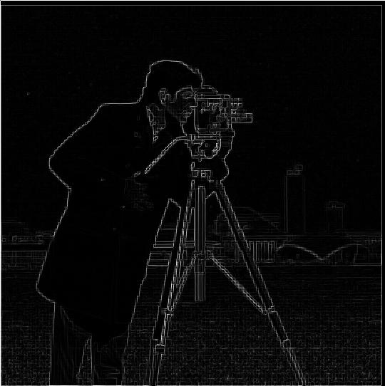
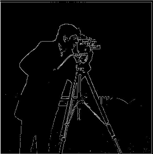
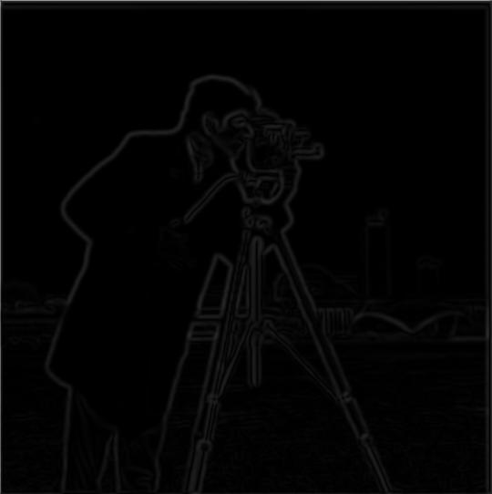
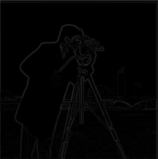
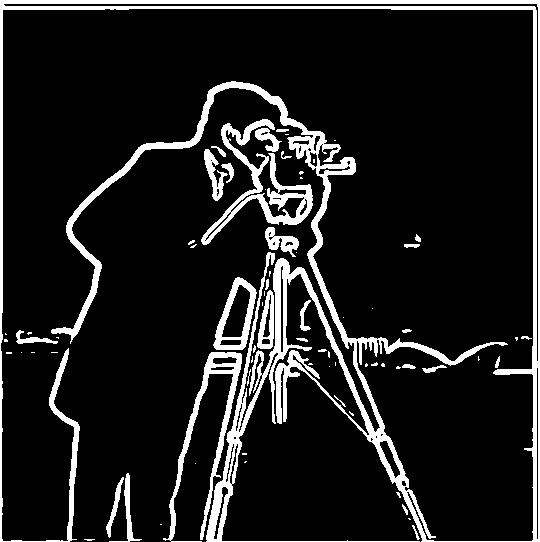
Given the derivative images with respect to both the x and y directions, we can compute the gradient-magnitude image (given by the square root of Dx^2 + Dy^2). However, there was some noise in the gradient magnitude image. Therefore, I normalized the gradient magnitude image and binarized the image (only consider pixels greater than 0.2 in value on a scale from 0 to 1) to take out the noise. For gradient magnitude normalization, I subtracted the minimum value from the image and divided the entire image by the maximum value minus the minimum value.

With a high screen brightness, one can see that binarizing the gradient magnitude image takes out some of the noise in the foreground (grass). However, the binarized image is still a bit noisy.

1.2

For this part, I used a Gaussian kernel to blur (low-pass filter) the input image. This way, there would be reduced noise in the derivative and gradient magnitude images. My kernel size was 15x15 with a standard deviation (sigma) of 2. This setup follows the convention of the kernel half-width being at least 3 times the standard deviation of the kernel.

As seen in the above pictures, the images for the respective operations are less noisy. For the binarized gradient magnitude image, I considered pixels with value > 0.07 on a scale from 0 to 1. The binarized magnitude image has cleaner edges compared to the image derived from a non-blurred input.

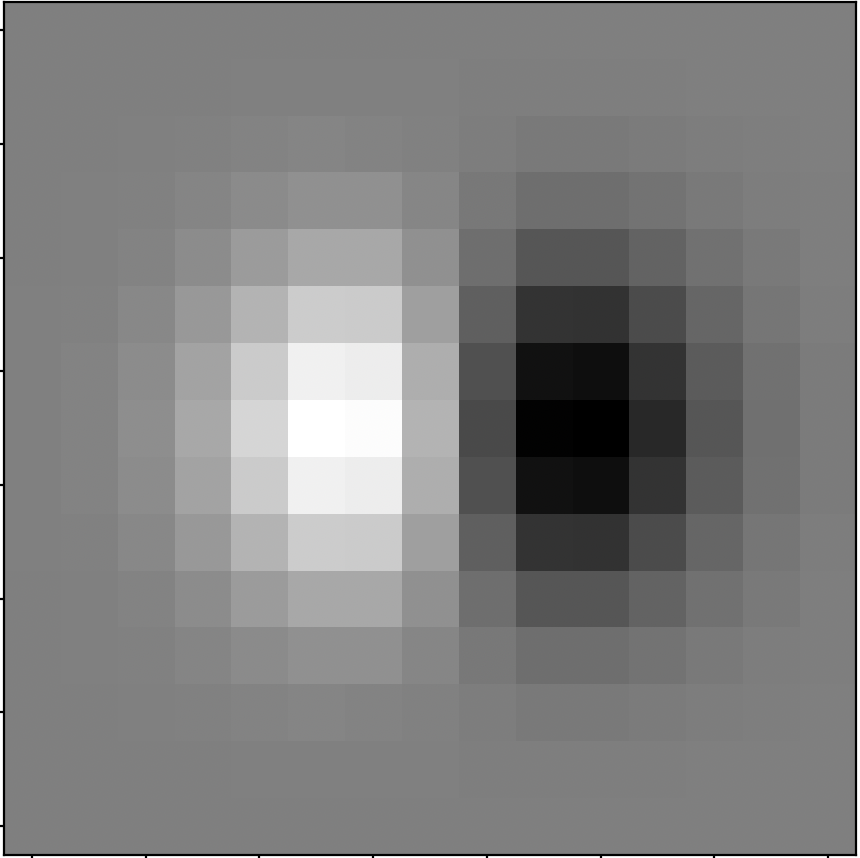
Now, instead of blurring the input first and then applying the finite difference operators, we can convolve the gaussian kernel with the finite difference operators first. This switch of operations is allowed by the associative property of convolution. Thus, we can convolve the input with the derivatives of the gaussian kernel (in x and y) to obtain the same results as above:

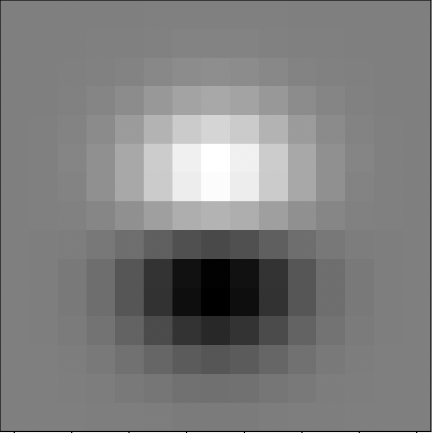
As seen above, the results are essentially identical to the previous results in 1.2. These results were obtained the following filters (for x and y):

Part 2

This part of the project explores the power of frequencies with respect to image data.

2.1

For this part, I was tasked with image sharpening. The results of Part 1 showed that convolving an input image with a gaussian kernel results in a blurred image. This blurring relates to the low-pass filtering that a gaussian kernel does. The blurred image is the original image minus some higher frequency details (image sharpness). Therefore, we can derive an unsharp mask filter (image sharpening filter) using a gaussian kernel. If a gaussian kernel low-pass filters an image (i.e. takes away high frequency details), we can subtract the low-passed image from the original image to obtain the high frequency details. If we scale the high frequencies and add them back to the original image, we get an image that emphasizes sharpness. As a note, the high frequencies are scaled by a constant factor of ⍺.

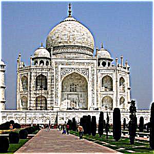
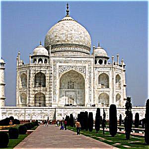
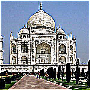
The first test image is one of the Taj Mahal. The unsharp mask filter described above was applied to each channel of the input image for best results. For all images in this part, I used a gaussian kernel with width 15 and standard deviation 2 for the unsharp mask filter.

By applying the logic stated above, the following results were obtained:

These images show that for greater values of alpha, the high-frequency details of the original image (taj.jpg) are emphasized more.

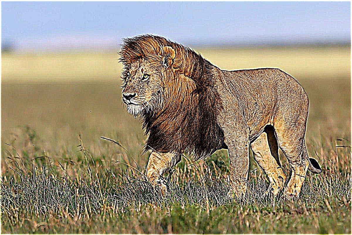
I tested out this image sharpening technique with another input image:

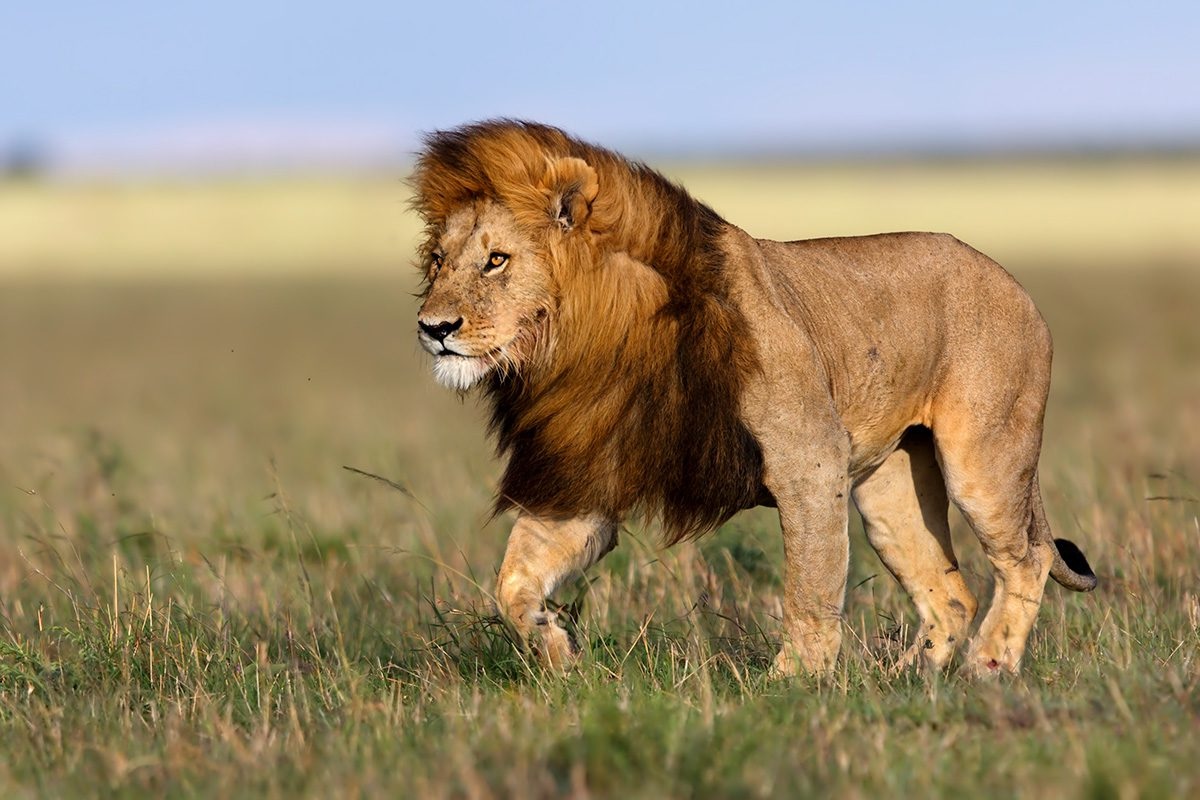
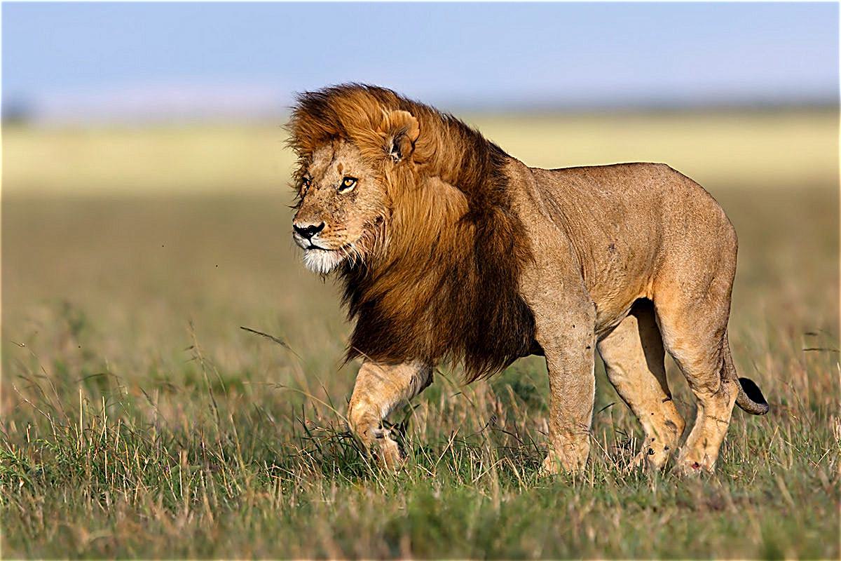
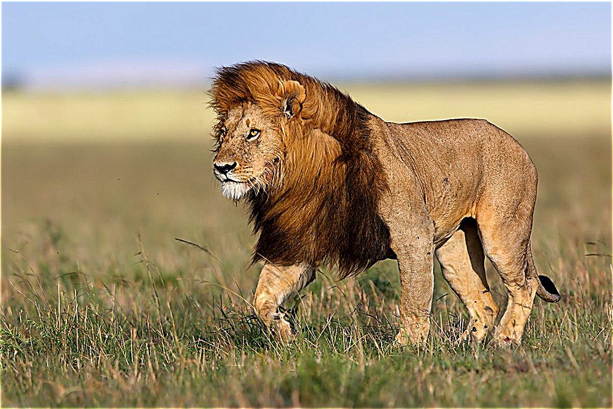
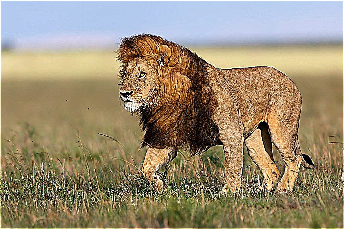
The above series of images display that the higher frequency components of the input image (i.e. the mane, fur, whiskers) are emphasized further with greater alpha values.

I also tested out blurring an already sharp image, and adding details back with the unsharp mask filter. To blur the input image, I used a gaussian kernel with width 15 and standard deviation 2.

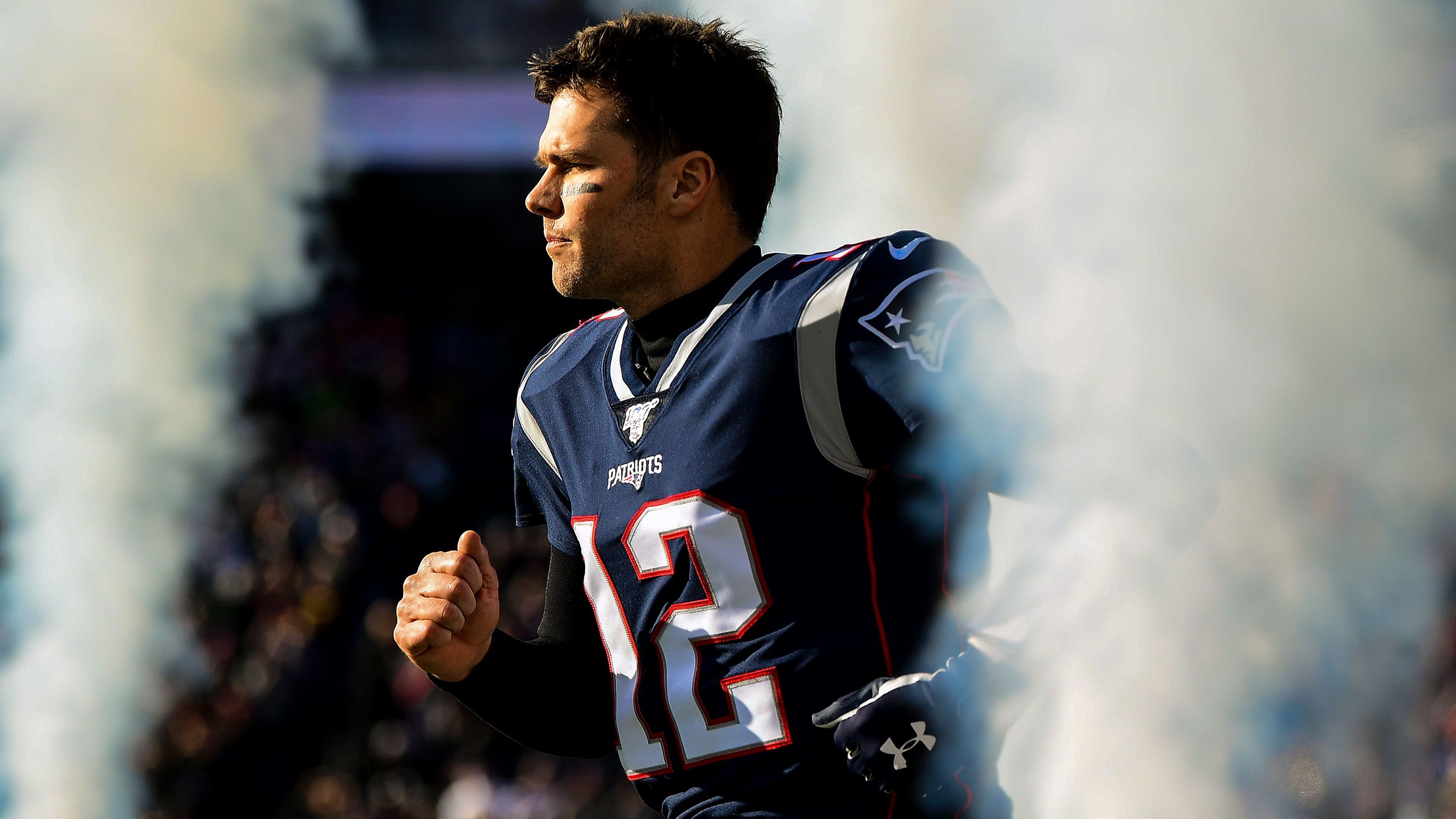
The following are attempts to recover the sharpness of the input image:

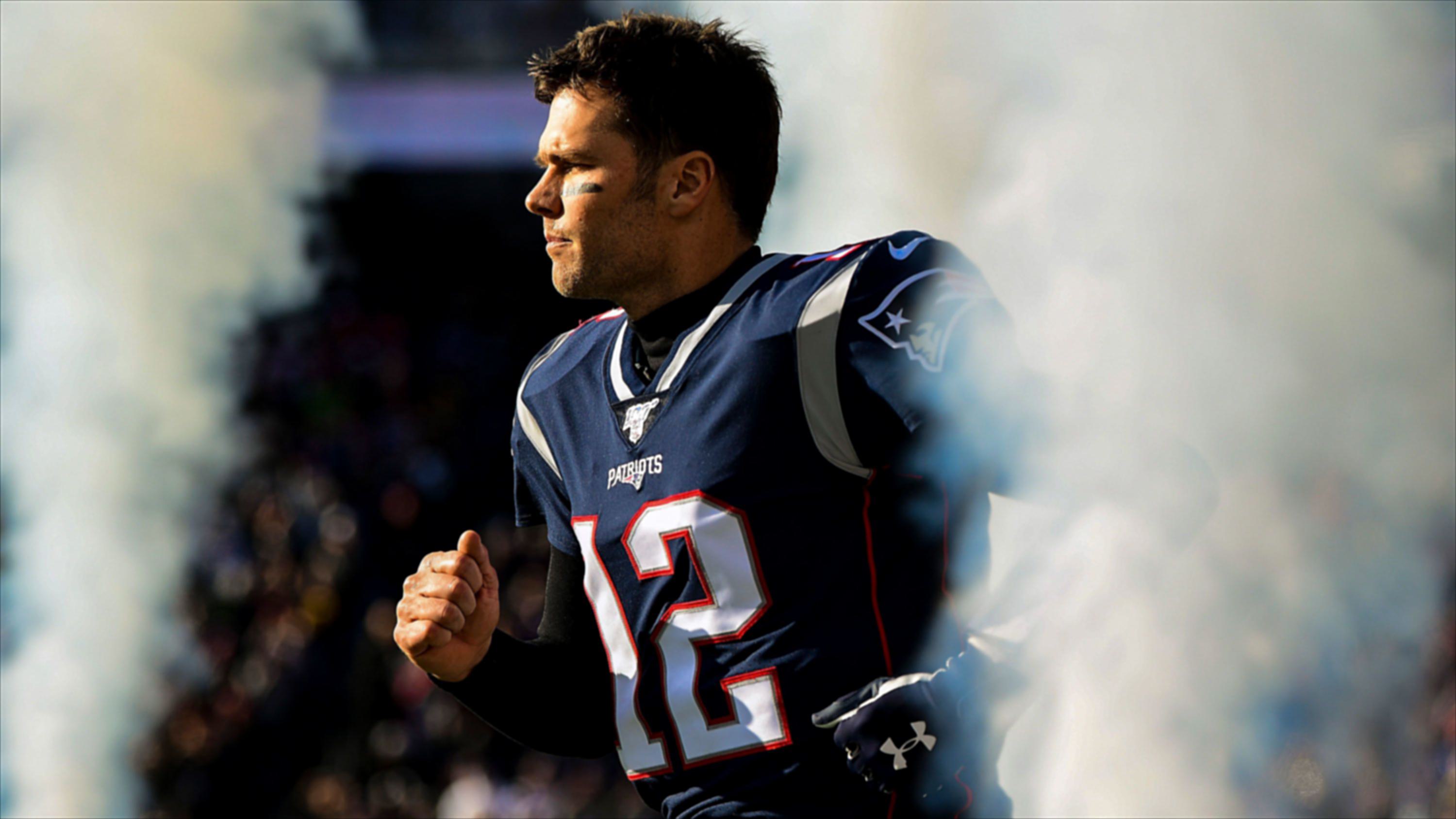
The results show that using some ⍺ | 2 < ⍺ < 4 for the unsharp mask filter would produce the ideal sharpness.

2.2

For this part of the project, I was tasked with producing hybrid images. Low-pass filtering one image would yield a low-frequency image that is more visible at a distance. High-pass filtering another image would yield a high-frequency image that is more visible close up. Averaging the low-frequencies of one image and the high frequencies of another image would result in a hybrid image (something that is perceived differently at varying distances).

I first tested out the hybrid-image technique on the provided Derek and Nutmeg example. I used gaussian kernels with σ=10 and width 61 for both low-pass and high pass filtering. For all examples in this part, I used the provided alignment code to align the two input images.

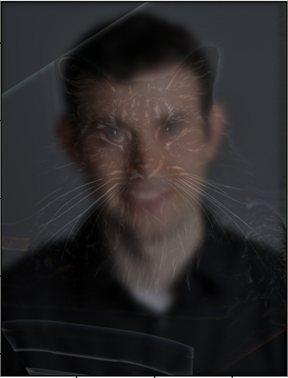
For the bells and whistles component of this part, I used the color versions of both input images for best results. As seen above, Nutmeg (the cat) is visible at a close distance, while Derek becomes more visible further from the screen.

I tested out the hybrid image approach on two sets of new images. For both sets, I used σ=10 for the low frequency input and σ=7 for the high frequency input. For both sets, the gaussian kernel for each filter had a width of (6 * σ + 1).

This first set was a failure:

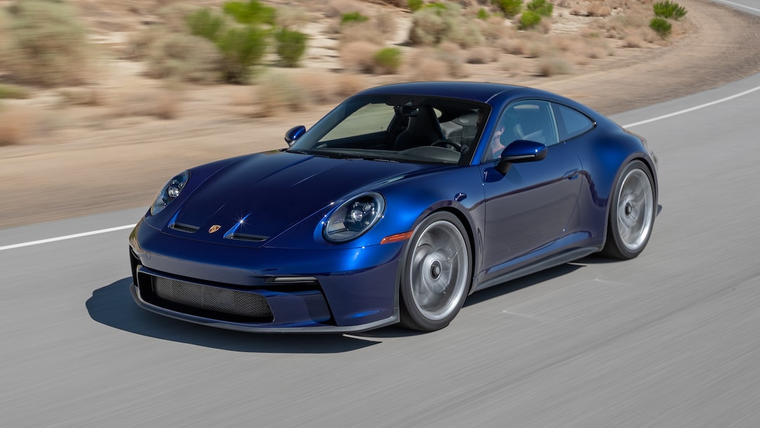
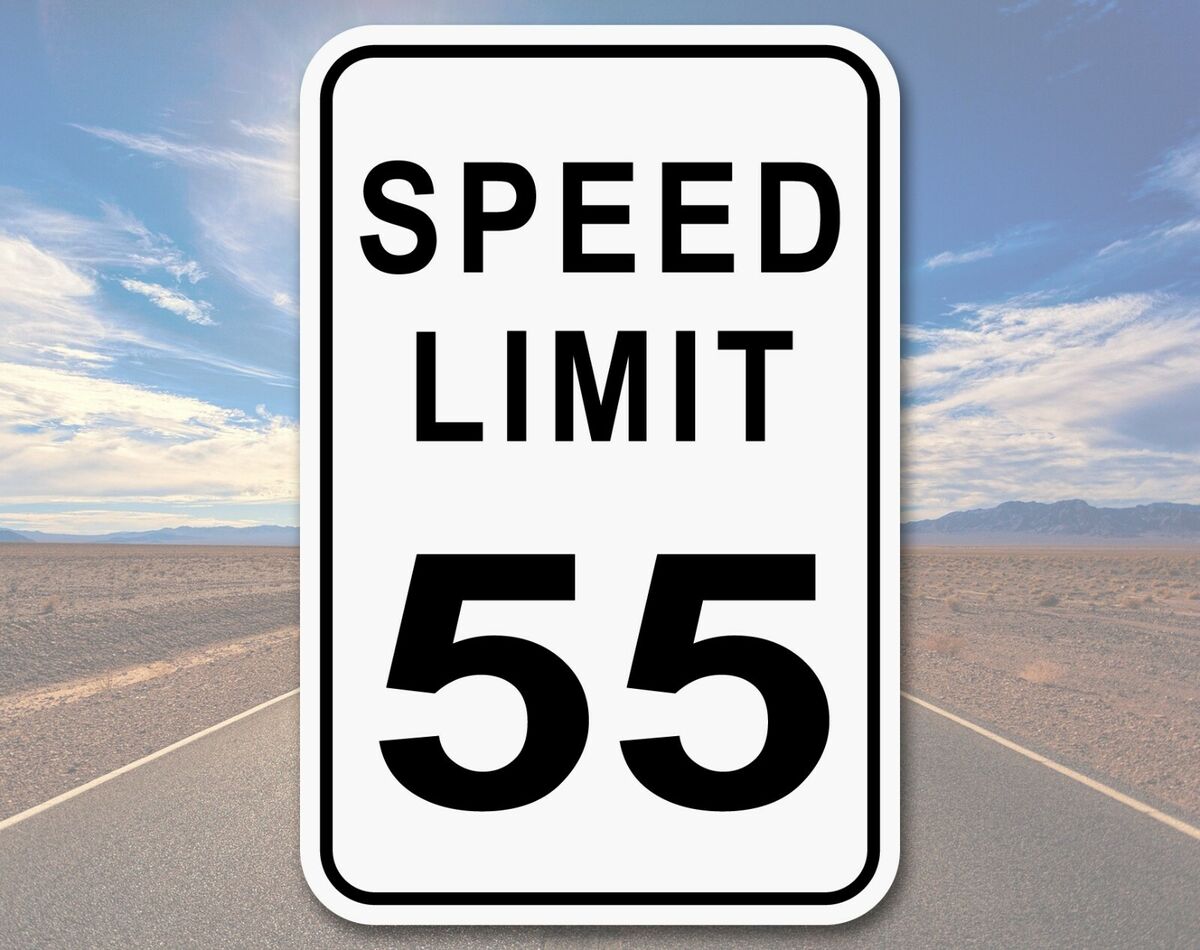
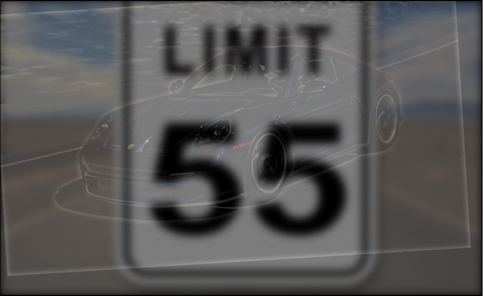
As seen above, the hybridization technique doesn’t work properly due to the dominant black outlines and font of the low frequency image. It is also difficult to align the two images properly (extreme differences in shape).

My favorite hybrid image was more of a success:

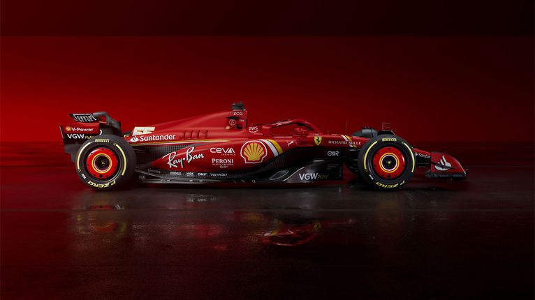
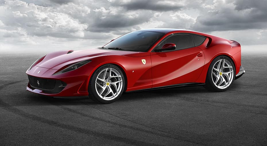
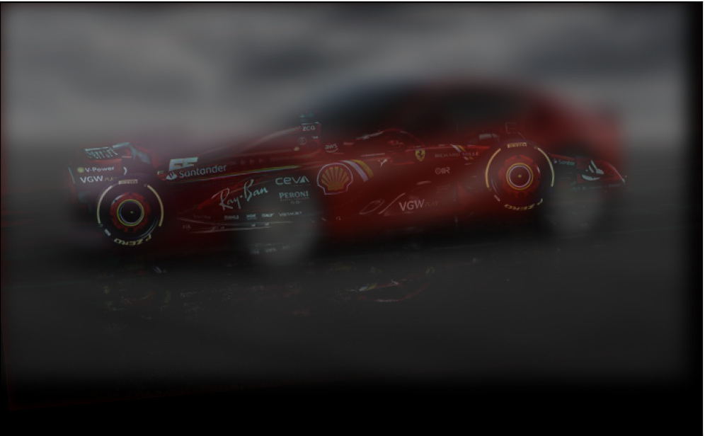
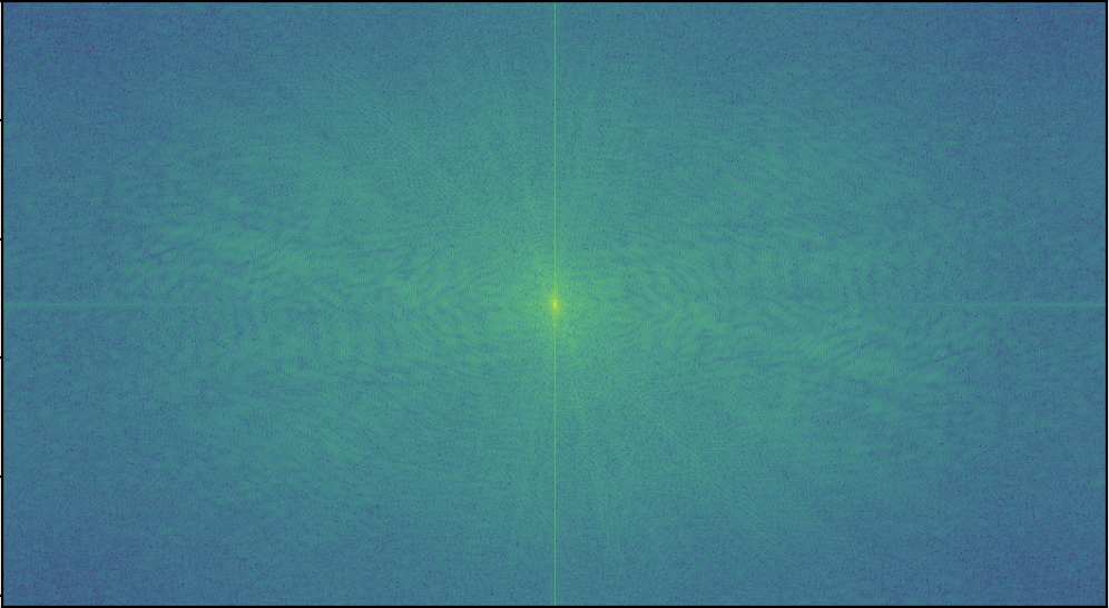
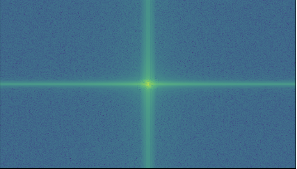
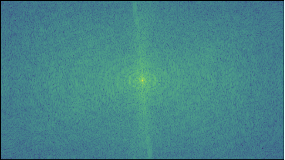
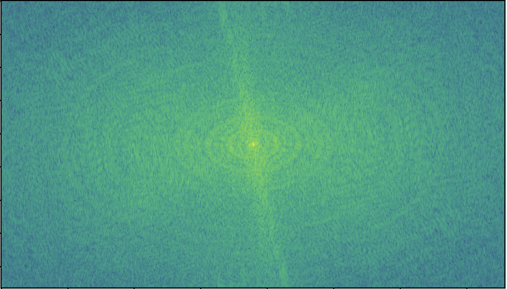
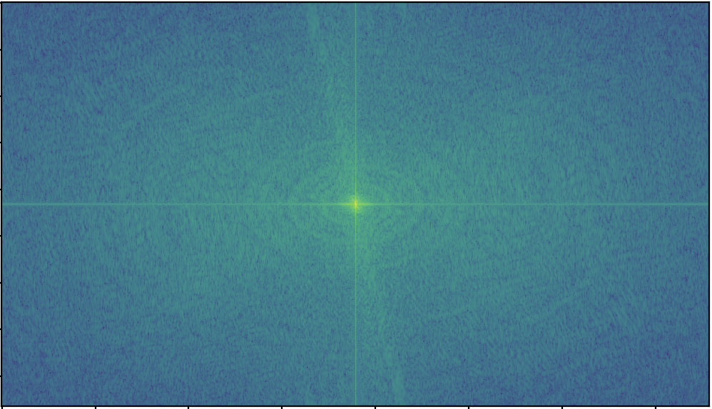
The results are intriguing when considering the Fourier domain. I visualized the input images, low and high-passed images, and the output image in the Fourier domain:

2.3-2.4

For these parts, I was tasked with performing multi-resolution blending. This process involves taking two input images (with a mask) and producing a blended combination of both images. This blended combination should be relatively seamless and not have any obvious artifacts.

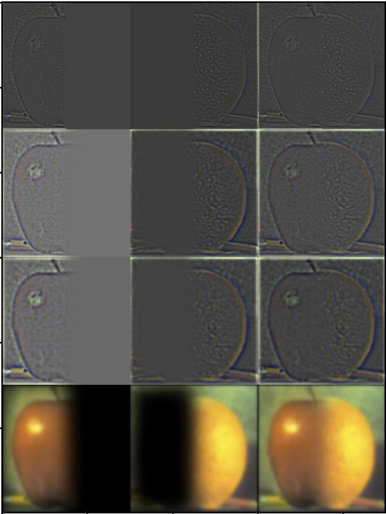
The first step of this multi-resolution blending process was to construct gaussian stacks of both input images. The gaussian stacks were constructed by repeatedly low-pass filtering an image (using a gaussian kernel). To construct a gaussian stack of all input image, I used a gaussian kernel of size 15, with σ=2.

The construction of the gaussian stack for each image helped with creating the laplacian stack for each image. I constructed the laplacian stack by subtracting the second level of the gaussian stack from the first level of the gaussian stack and so on. Essentially, the laplacian stack consists of the sub-band images (higher frequency details lost between levels of the gaussian stack). The last level of the laplacian stack is taken from the last level of the gaussian stack.

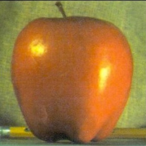
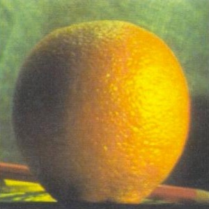
To construct a properly blended image, I also used a mask for both input images. For the apple + orange example, I used a horizontal step function as a mask. (1s in the left half, 0s in the right half). I multiplied each level of the mask gaussian stack with the left image, and the opposite of the mask with the right image (left * mask + right * (1 - mask)). I also constructed a gaussian stack for the mask using a gaussian kernel of size 121, with σ=20. This way, the blended image would have a less visible seam.

Here are my results for the apple + orange example:

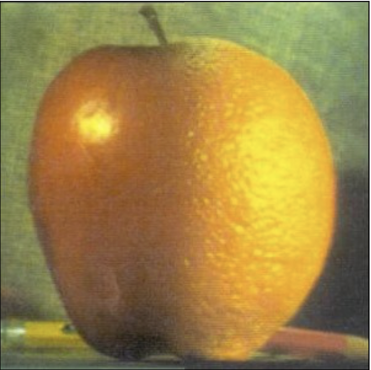
I tested out the image blending technique with a few other images. For this first set, I used an irregular mask (circle mask). For the gaussian stack of the circular mask, I used a kernel size of 61, with σ=10:

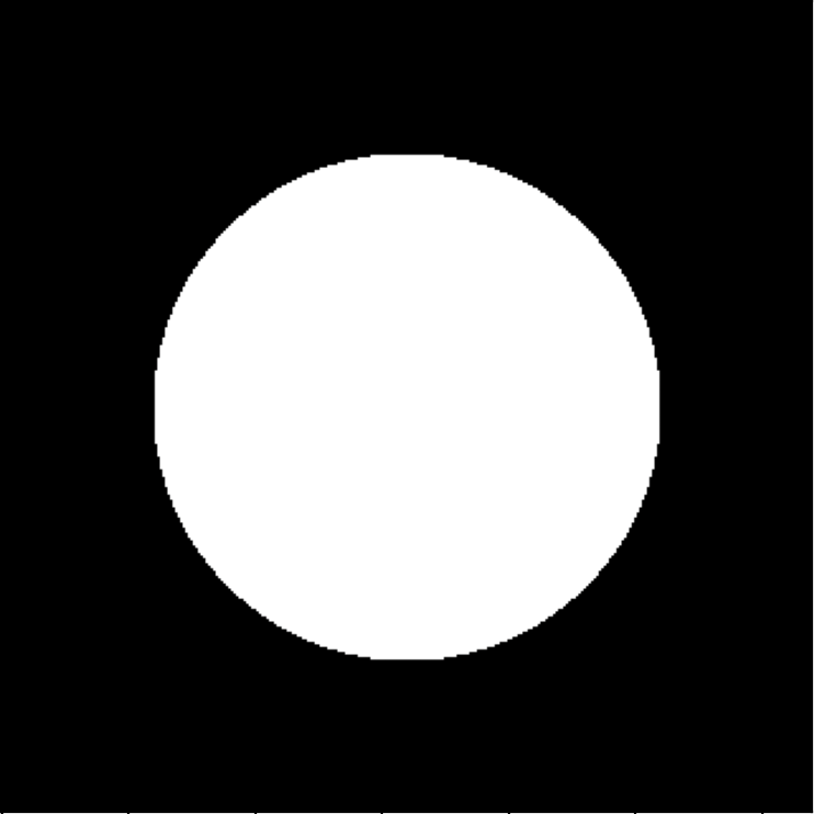
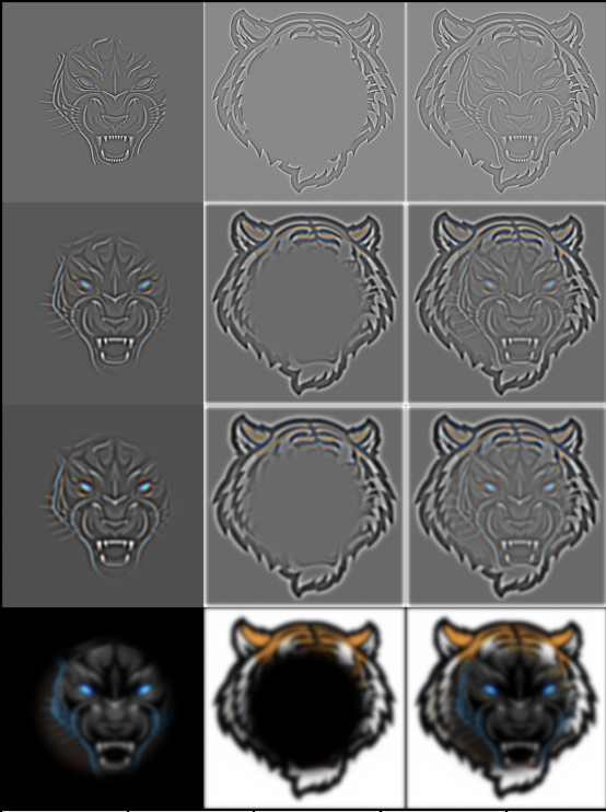
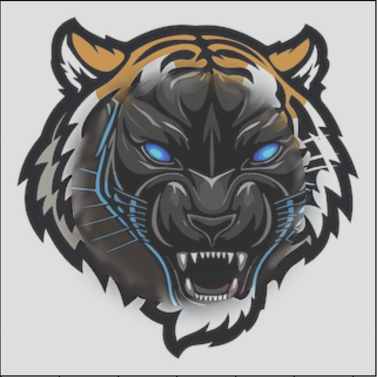
Another example with the circular mask. For the gaussian stack of this circular mask, I used a kernel size of 121, with σ=20:

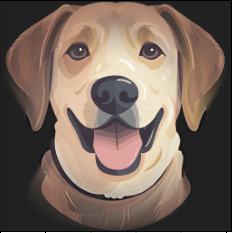
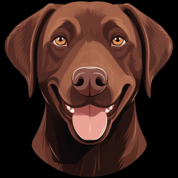
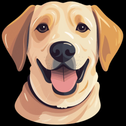
Here, the combined image has the ears and neck area of the brown lab, and the face of the yellow lab.