Goal

The goal of this assignment is to experiment with image transformations. In particular, this project involves using image transformations to generate image mosaics. The first half (Section A) deals with the basics of image transformations (i.e. homographies). The second half (Section B) delves into automatic mosaic generation.

Section A

Image Transformation Basics

Part 1

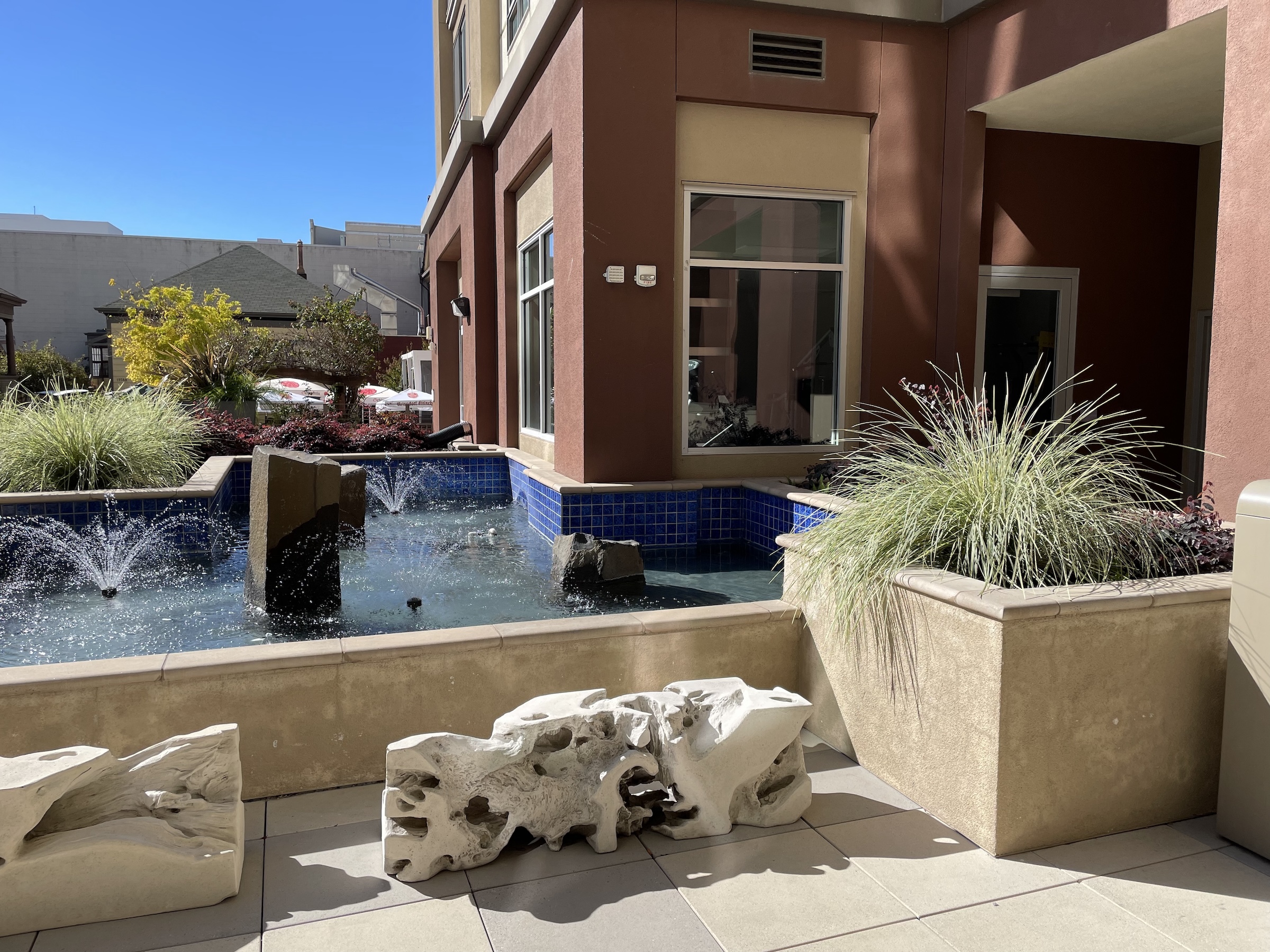
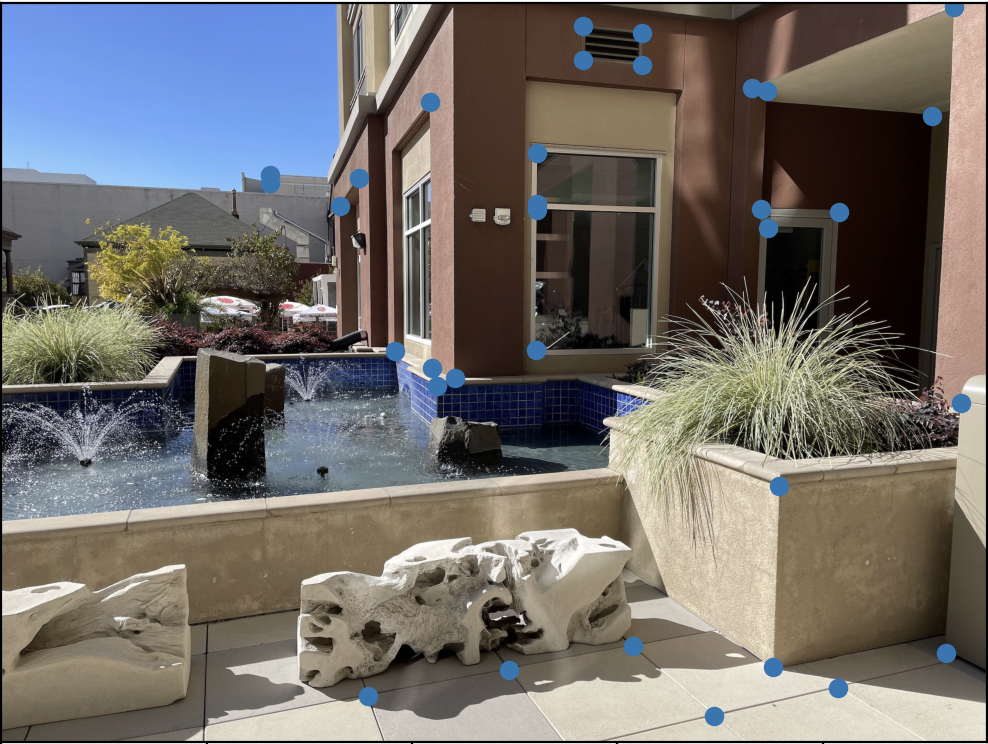
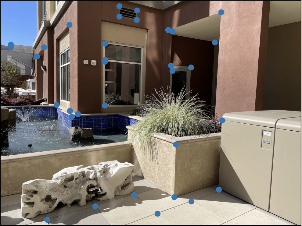
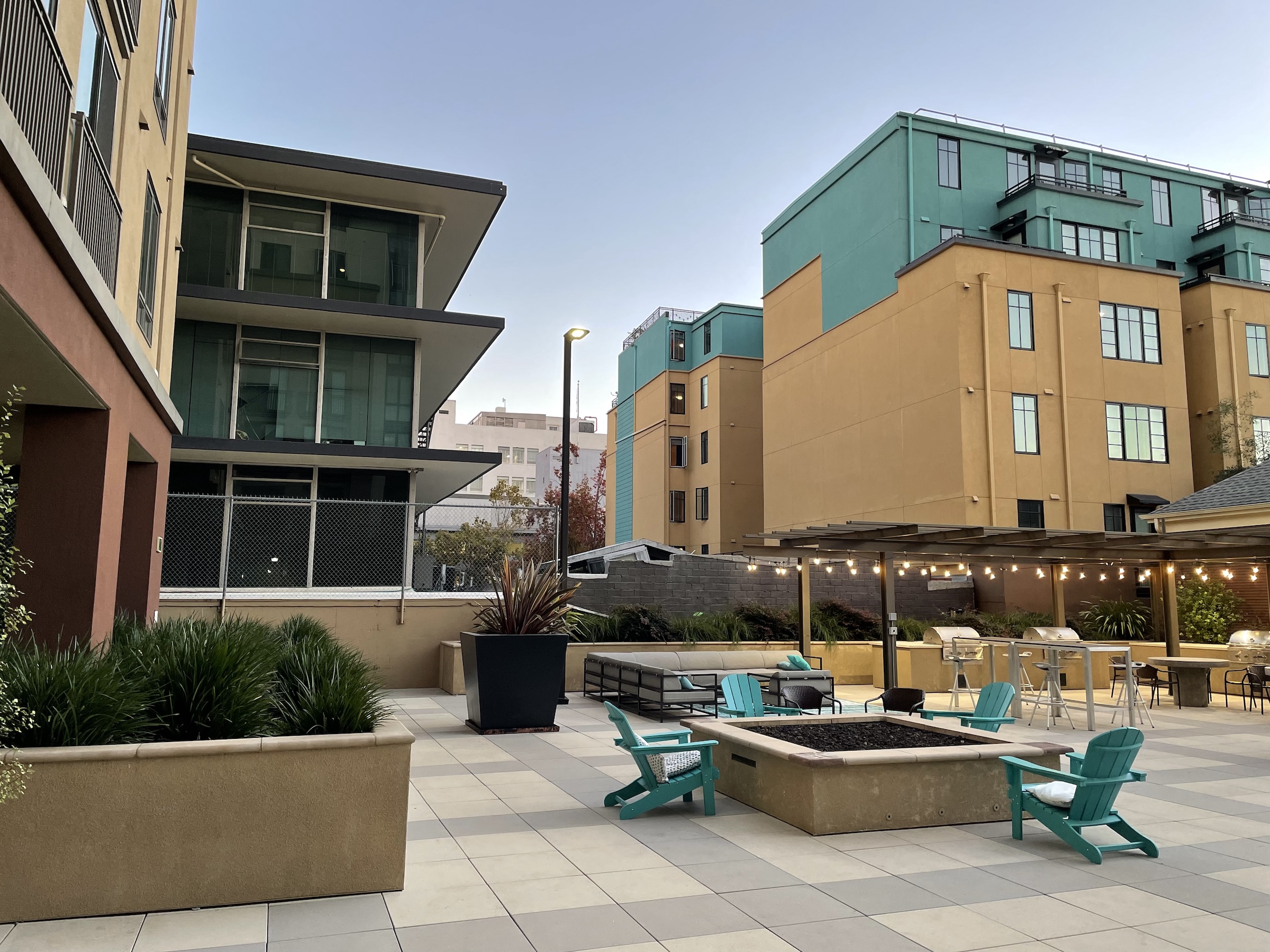
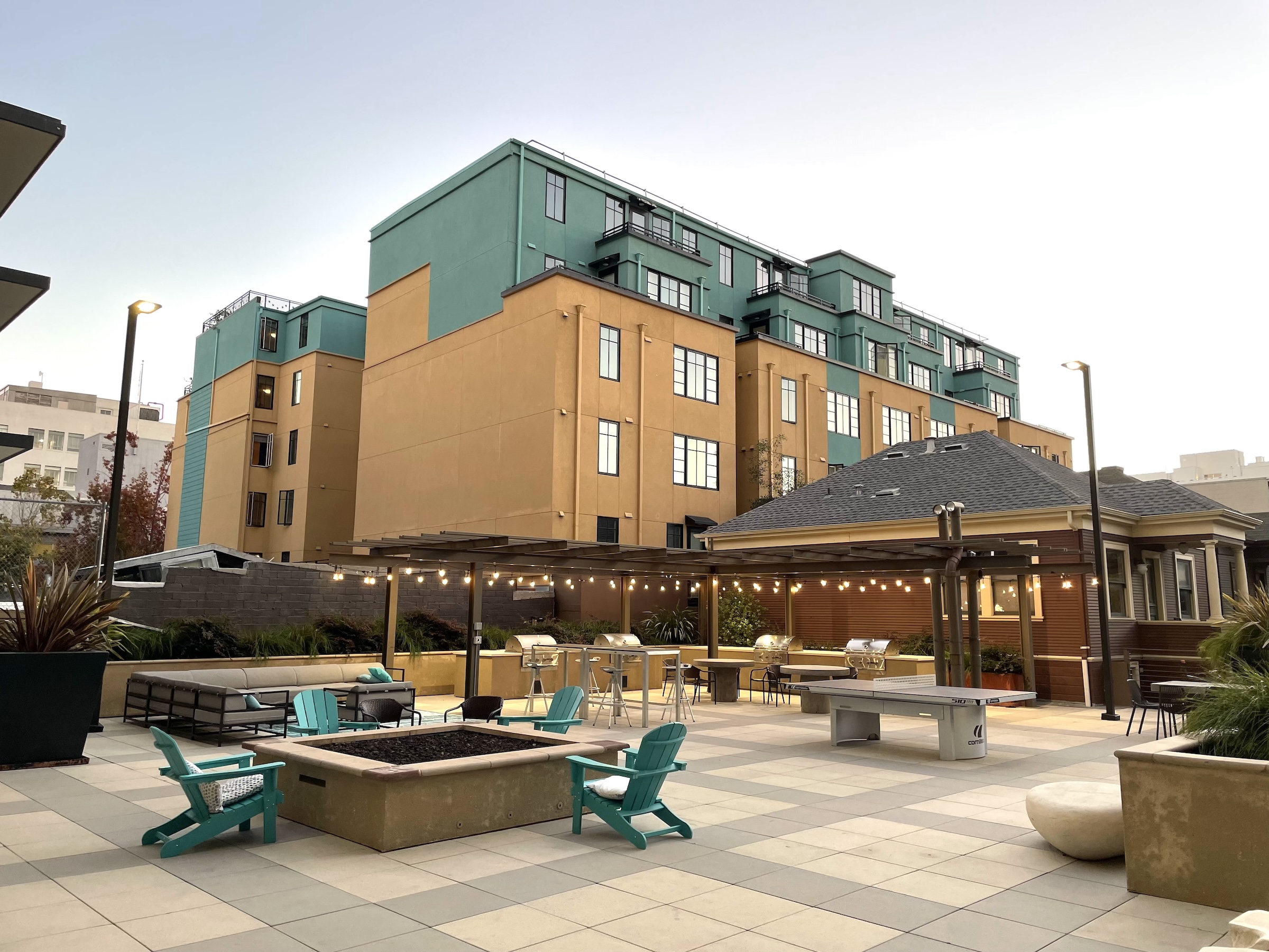
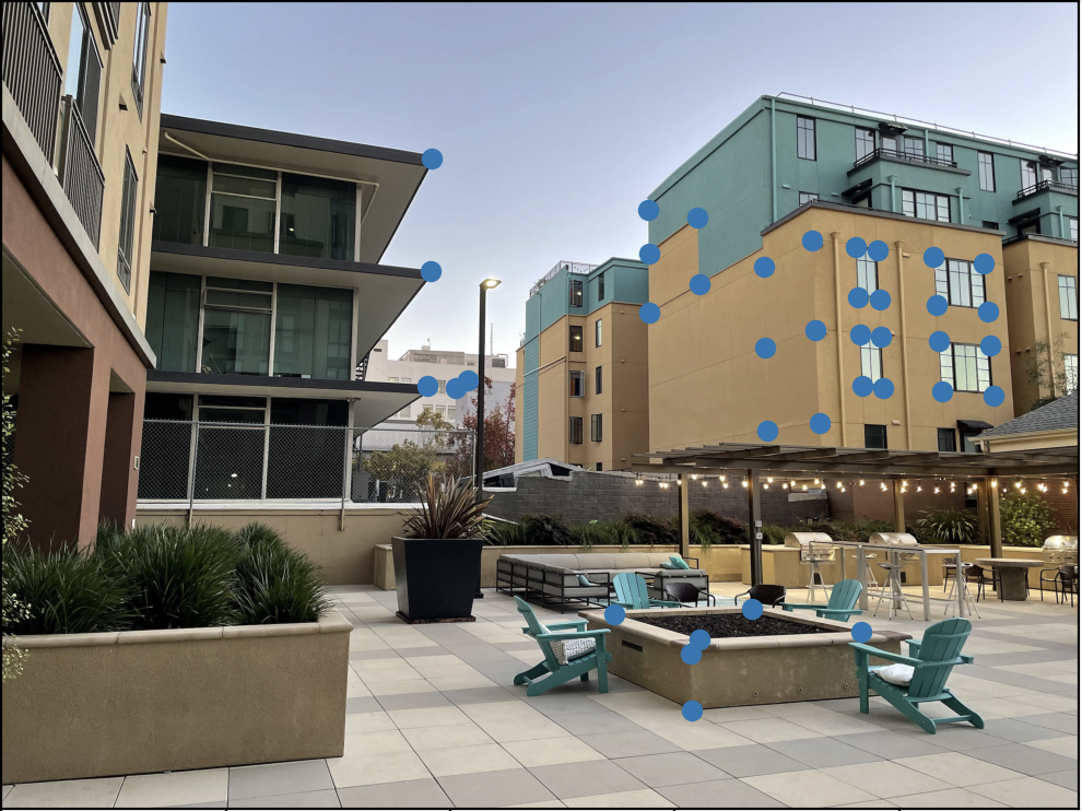
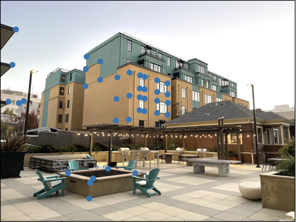
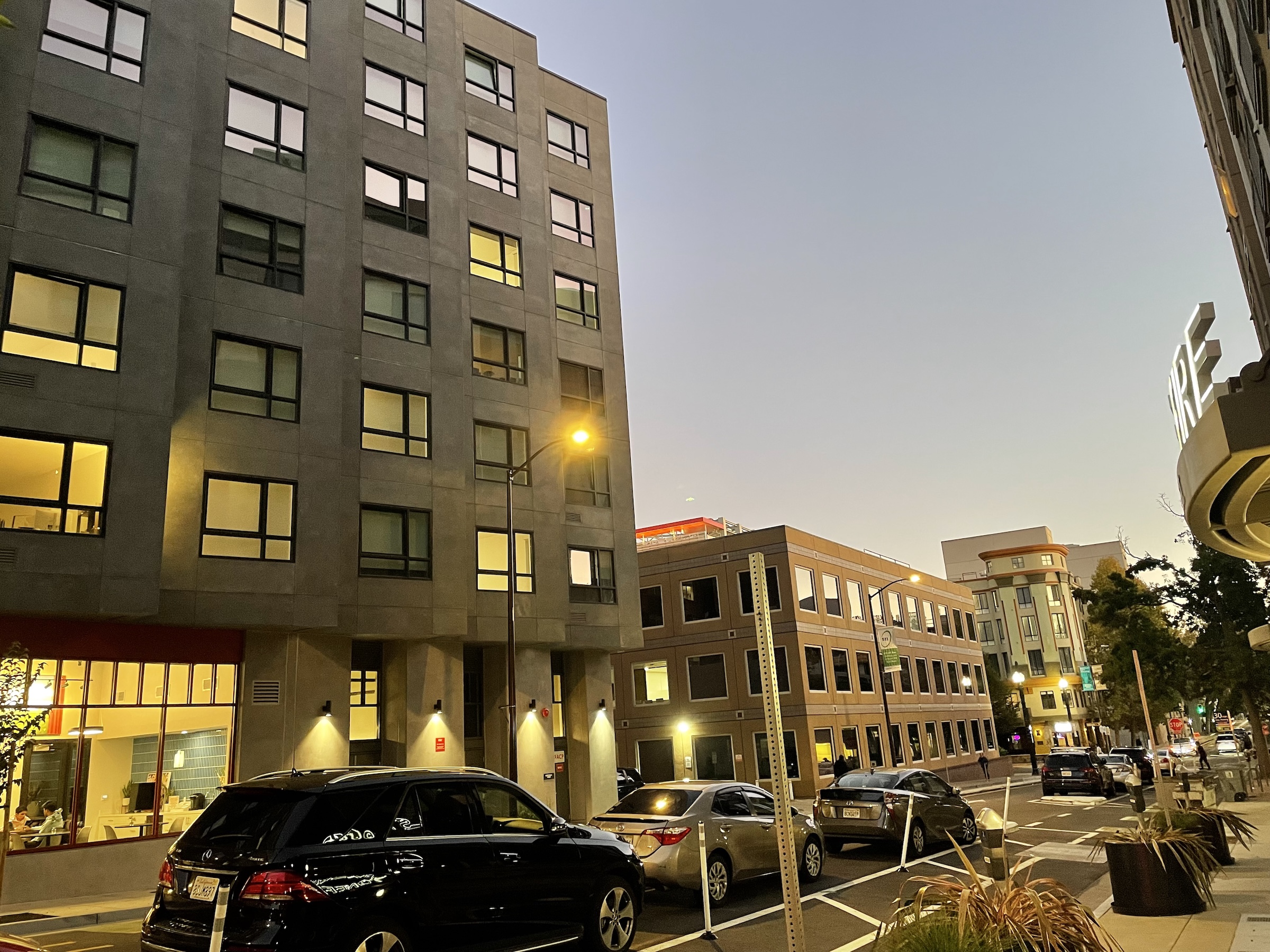
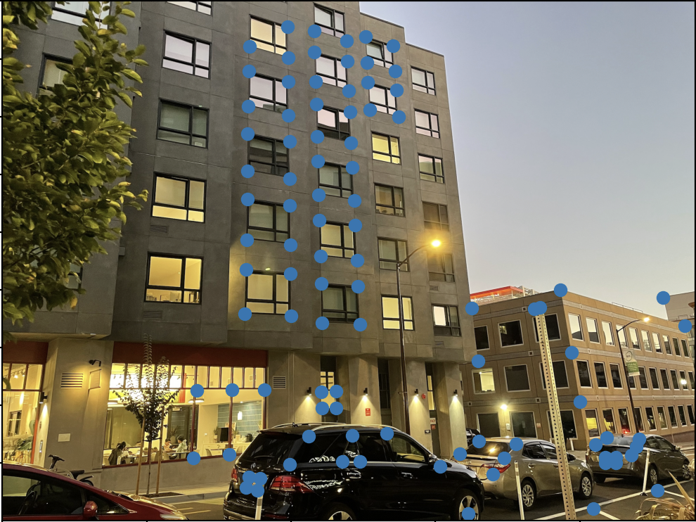
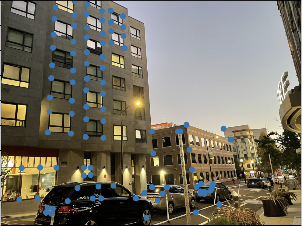
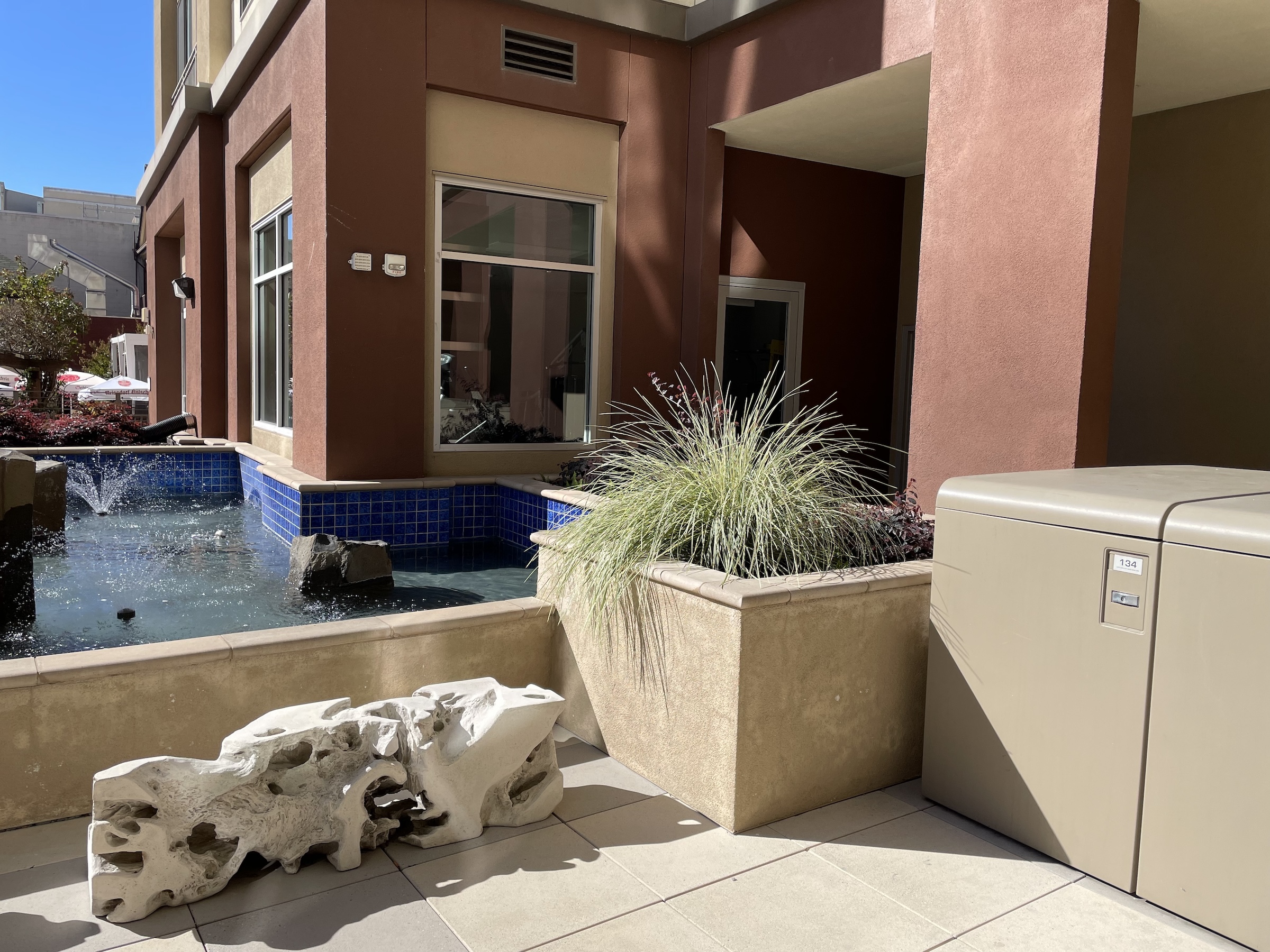
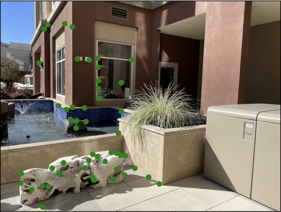
This part of the project involved taking pictures that could be part of the same mosaic (maintaining the same center of projection). I also marked correspondences between images using the provided online tool.

Set 1:

Set 2:

Set 3:

Part 2

This part of the project involved computing/recovering homographies. A homography is a transformation that maps one projection plane to another (although they ideally must share the same center of projection).

In order to compute a homography matrix H, I solved the least squares estimate for the elements of H based on the below derivation.

*Note p’ is the point in the target image, and p is the point in the source image

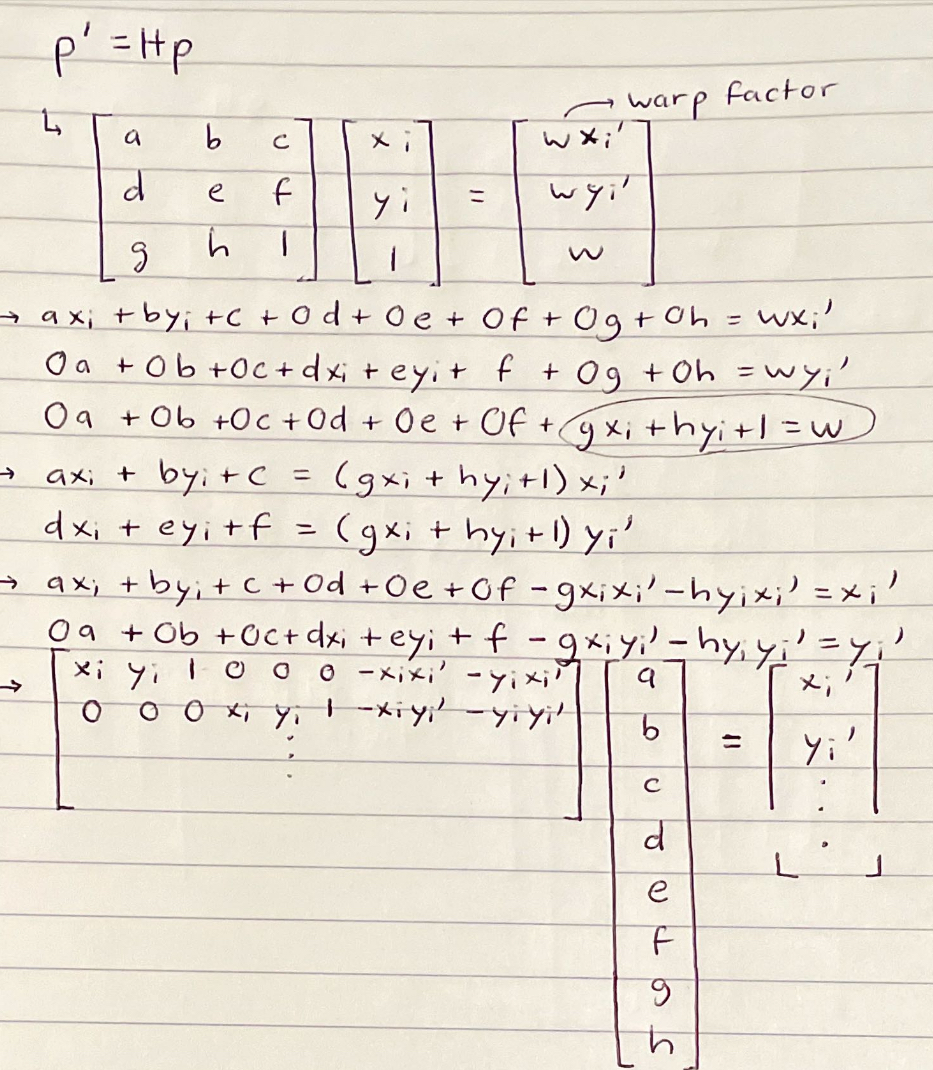
*As a note, for xi’, the prime (‘) denotes a coordinate in the target domain (i.e. image 2), while xi is a coordinate in the source domain (i.e. image 1). The least squares estimate is constructed based off of all the (xi, yi), (xi’, yi’) correspondence pairs between images. When applying the homography to correspondences (i.e. a point in the source image), it is important to note that the transformed vector contains a warp factor for each coordinate. Dividing by the warp factor yields the true estimated point in the target image.

Part 3

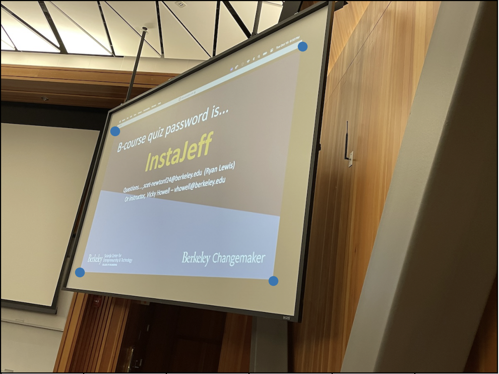
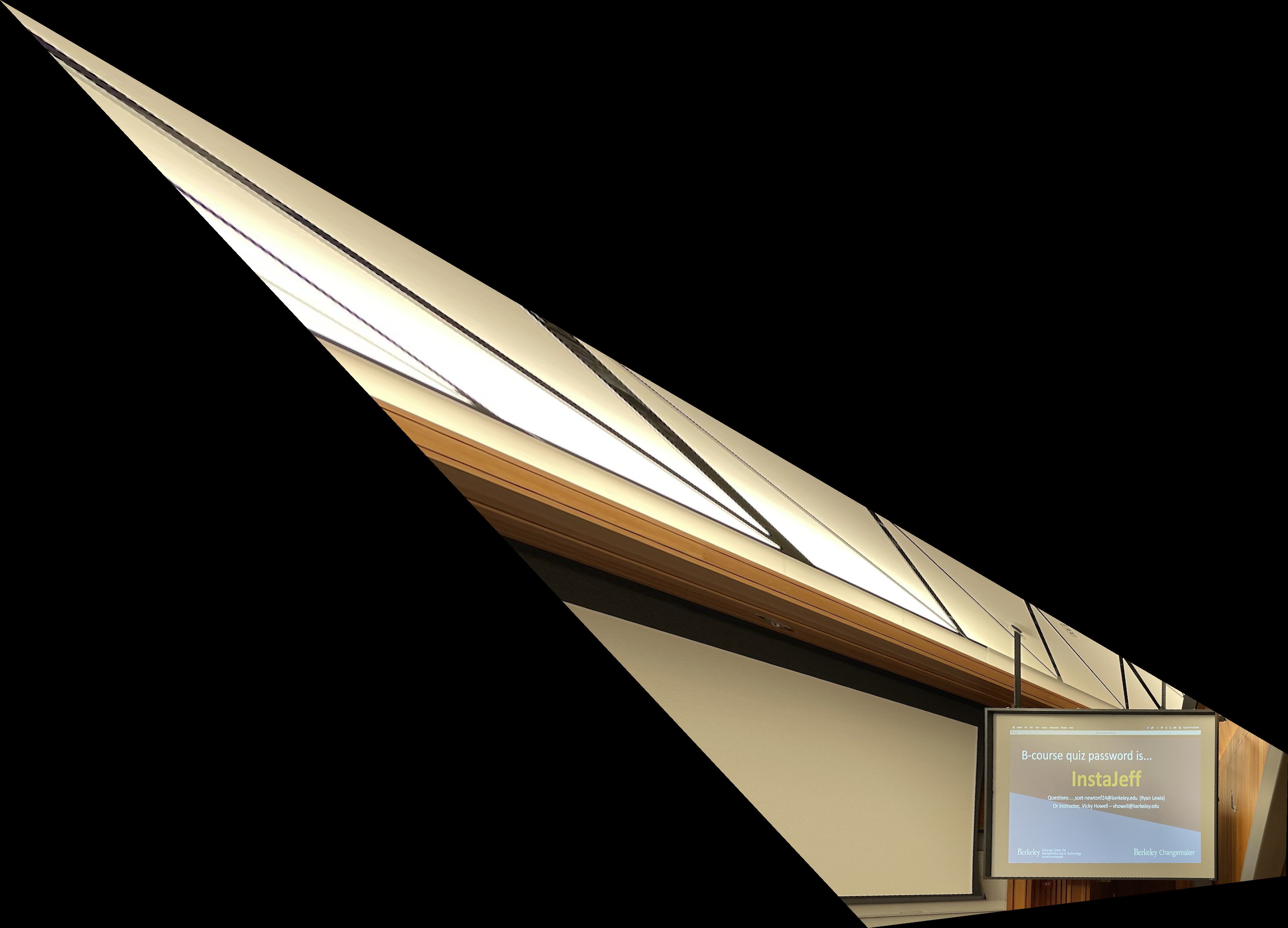
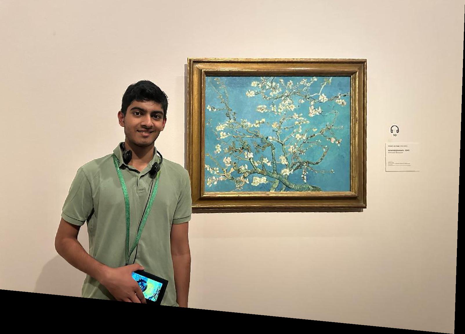
This part of the project involved using the calculated homographies (from the method described in Part 2) to warp reference images. In particular, the homography transformation can be used to “rectify” an image, or turn a perceived non-rectangular feature (due to camera location and feature location/orientation) into a rectangular feature.

Here are my results for image rectification:

Example 1:

Example 2:

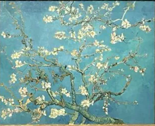
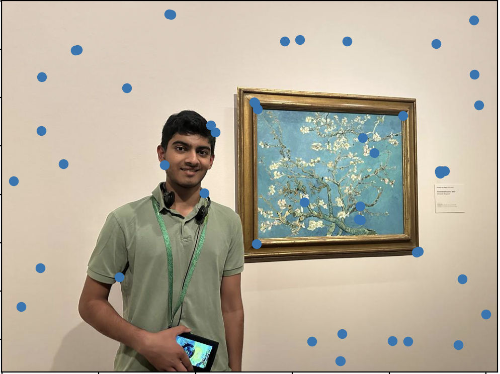
(*for the art connoisseur, the second example is me next to Van Gogh’s Almond Blossom)

Part 4

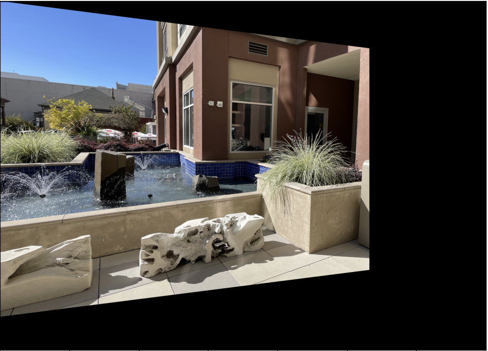
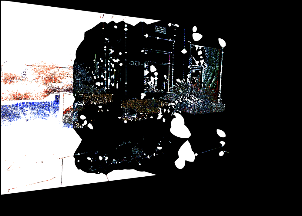
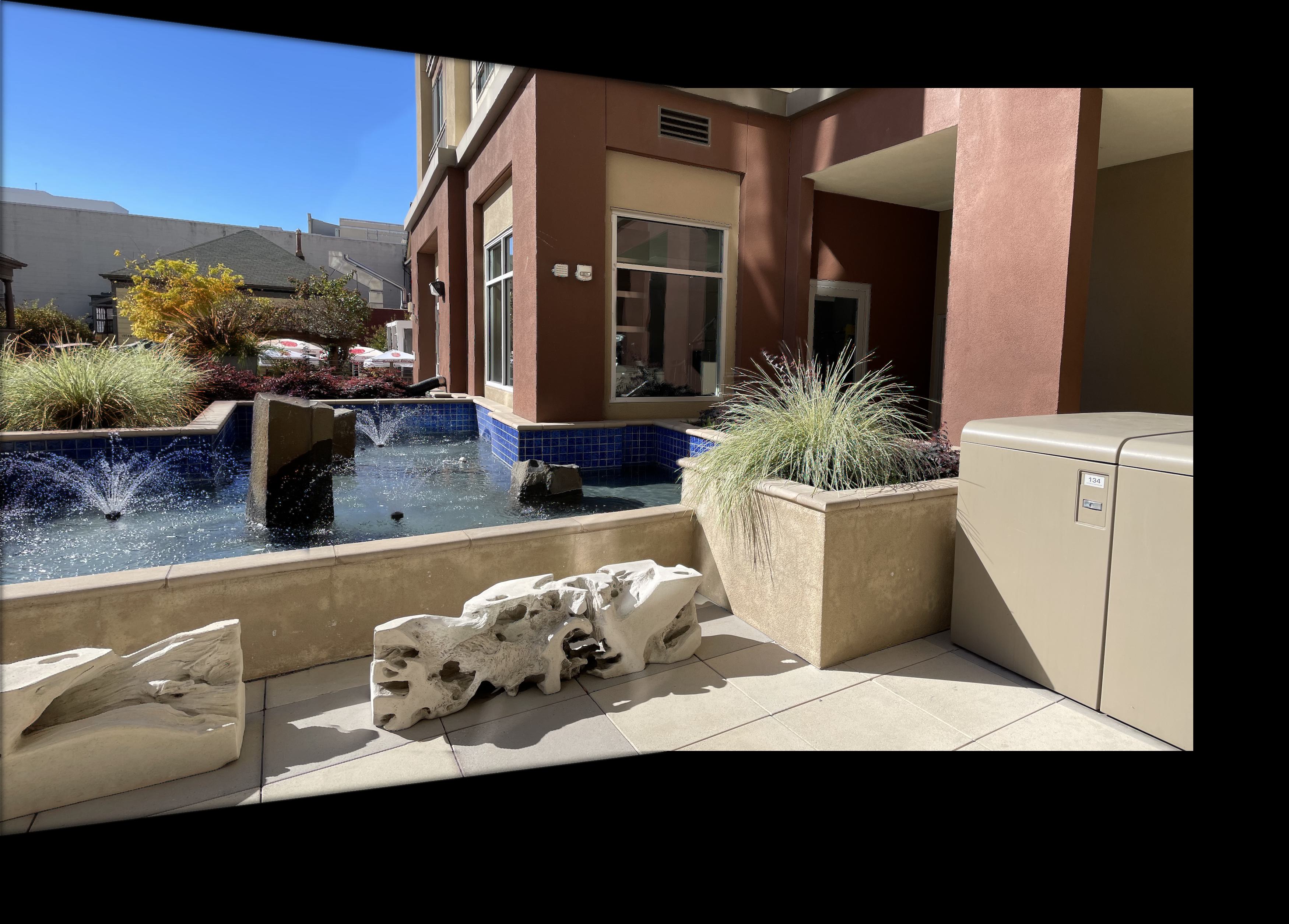
For this part, I was tasked with blending warped images into a complete mosaic (panorama). To do so, I first computed a homography matrix H based on the correspondences between the “left”and “right” image. Then, I warped each “left” image, based on its corners, to find the polygon corresponding to the warped image. Subsequently, I used the inverse warp/homography matrix H, to populate pixel values in the warped image with those from the original image.

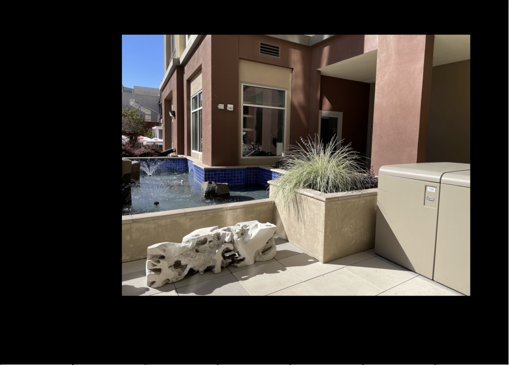
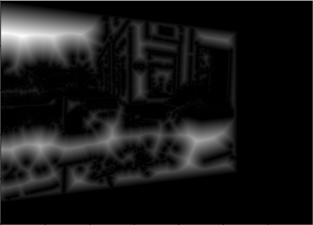
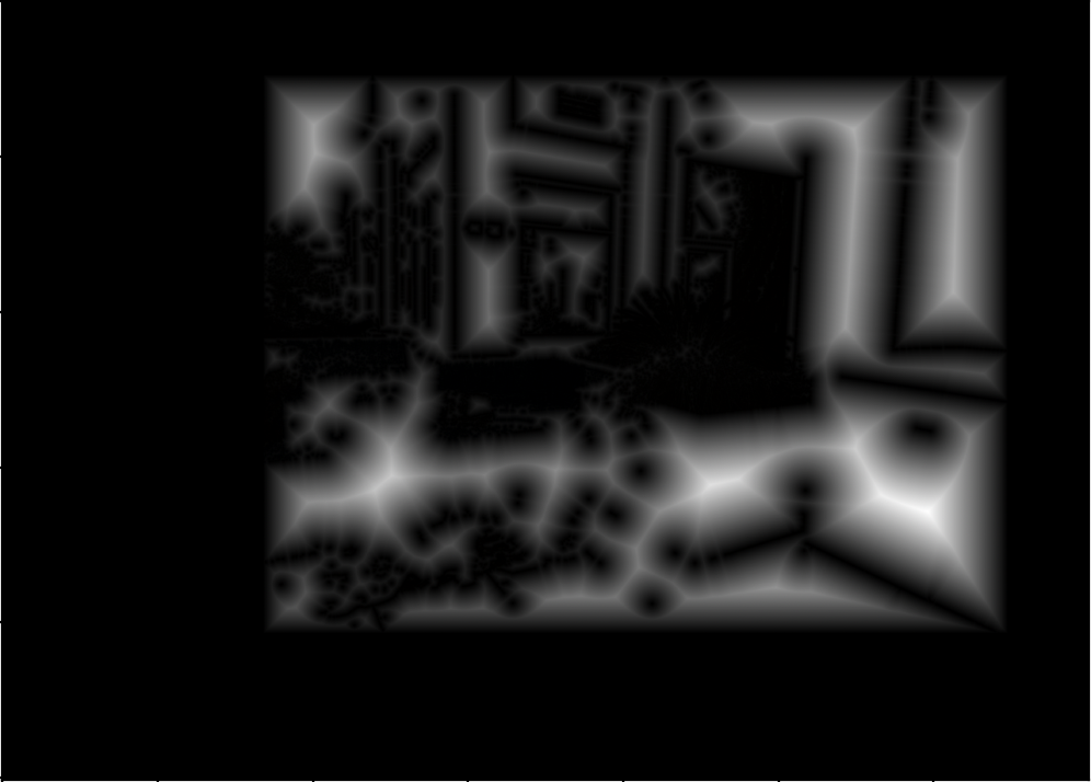
To combine the two images (transformed ”left” and original “right”) into a mosaic, I used the distance transform. I calculated the normalized distance transform (which estimates the distance from each pixel to the closest background pixel, or pixel with value 0) for each part of the mosaic. Then, I generated a normalized mask based on where the distance transform for the left image was greater than the distance transform for the right image (1 if greater, 0 otherwise). Using the code from Project 2 (Laplacian blending), I blended the two masked images into a complete mosaic. My results are below:

Example 1:

I repeated the same process described in detail above for two more sets of mosaics:

Example 2:

Example 3:

Section B

The previous section (Section A) involved a lot of manual work, especially for detecting correspondences in a way that would result in a decent mosaic. This section of the project delves into automated mosaic generation. Parts 1-3 follow this paper by Brown et al.

Part 1

This part involved detecting “Harris” corners, with the help of provided starter code. Here is an example:

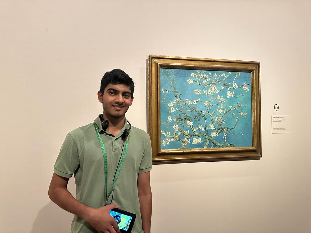
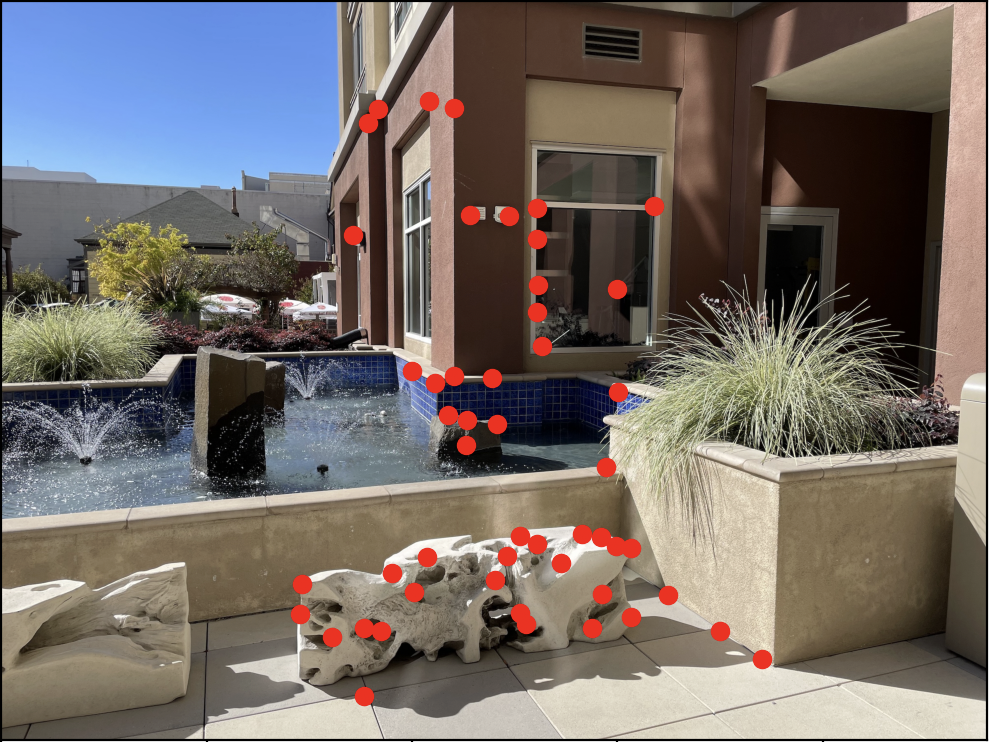
As seen above, the base Harris detection method is very sensitive, and finds way too many “corners” or interest points. In order to find more meaningful interest points, I implemented the Adaptive Non-Maximal Suppression method described in the paper linked above.

Adaptive Non-Maximal Suppression (ANMS) is a method for filtering the raw interest points gained from Harris corner detection. This method passes all top interest points that have the greatest corner strength of all neighboring points within a minimum radius r. I used a KD tree to store information about a given interest point and its corresponding neighbors. Then, I looked through the corner strengths of neighboring pixels. I kept increasing the search radius until I found a neighbor such that the given interest point’s corner strength is less than 0.9 (recommended c_robust according to the paper) of the neighbor’s corner strength. Upon finding a stronger neighbor, I recorded the minimum radius for the given interest point.

I sorted all corners by minimum radii, and selected the top corners as valid interest points:

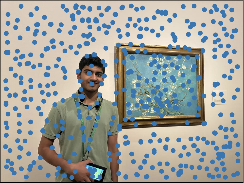
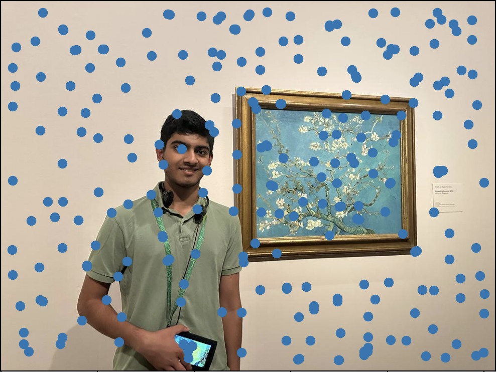
As seen above, using ANMS in addition to raw Harris corner detection allows for a more uniform and sparse set of interest points.

Part 2

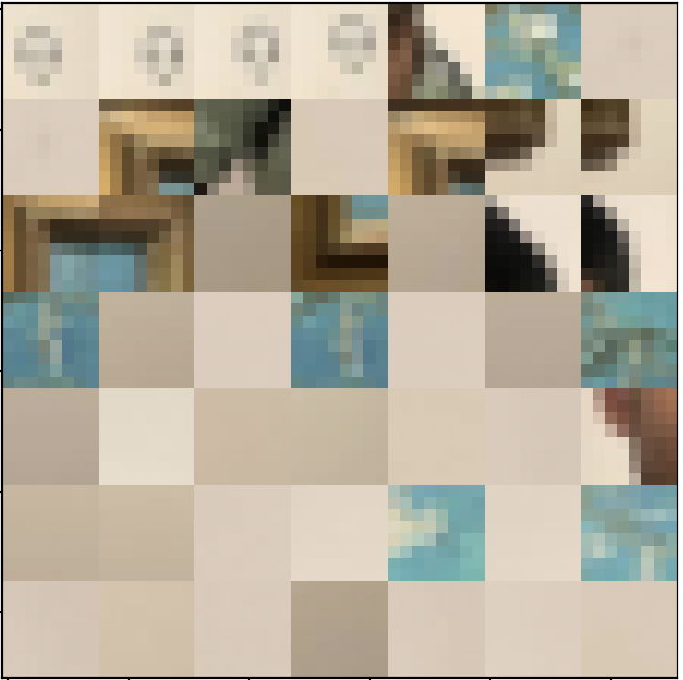
For this part, I extracted features for each interest point returned by the ANMS procedure. As described in the above linked paper from Brown et al, I collected 40x40 axis-aligned patches of pixels surrounding each ANMS interest point. Then, I downsampled each patch (with anti-aliasing/gaussian blurring) to obtain a “feature” for each interest point. I normalized each feature to account for bias and gain. Below is an example of collecting 49 features from running the ANMS procedure for 49 interest points:

Part 3

For this part, I used the aforementioned procedure of obtaining “features” from images to develop matches, or correspondences between images. After collecting features from both data images for the mosaic, I calculated the 2 nearest feature matches in the “right” image for each feature in the “left” image. To determine the similarity between features, I calculated the mean squared error between two features.

The 2-NN approach allowed me to use Lowe’s trick (comparing the best match to the second best match) to see if a matching feature was really that much better than a rival feature. In particular, I compared the ratio between mean squared errors of the two nearest features against a threshold. Using the ratio information, I was able to see if a correspondence was in fact valid.

The results are as follows:

Part 4

The procedure defined in Part 3 (above) may result in outliers, which can skew/disrupt the transformation of images into clean mosaics. To resolve this, I was tasked with implementing the Random Sample Consensus (RANSAC) method for robust homography calculation.

The RANSAC loop consists of four main steps:

1. Randomly sample 4 pairs of corresponding points (without replacement) from the collection of correspondences

2. Compute an exact homography matrix H that transforms the sample points from image 1 onto the sample points from image 2

3. Apply H matrix from step 2 to all the correspondences. Compute a set of inliers (subset of all correspondences), where the deviations between estimated corresponding points in image 2 and actual corresponding points in image 2 is below a threshold

4. Maintain the largest set of inliers. Compute the least squares estimate of the homography matrix H based on the largest set of inliers.

After acquiring a valid, robust homography matrix H, we can apply the mosaic generation steps outlined in Section A to generate an appropriate mosaic.

Part 5

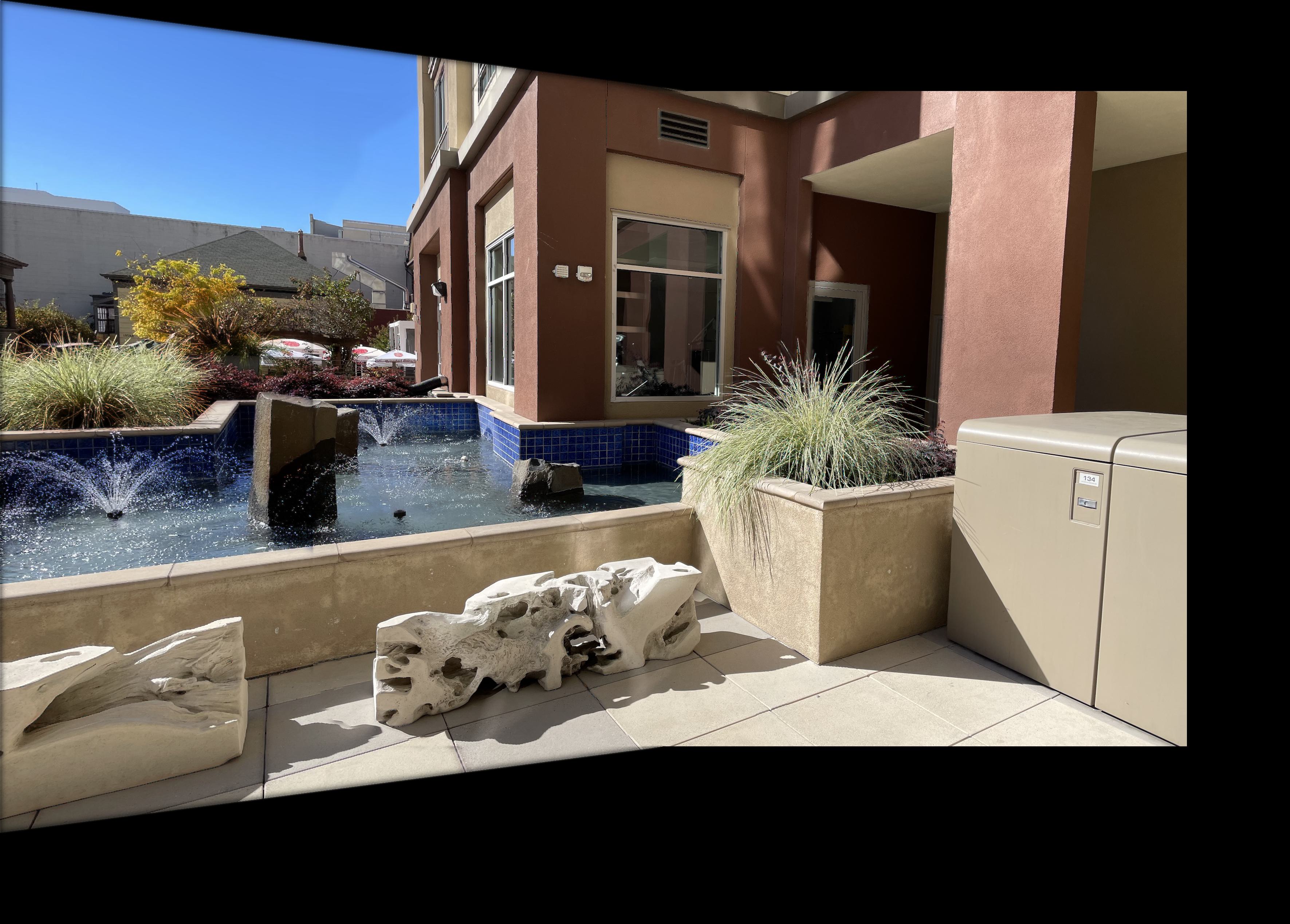
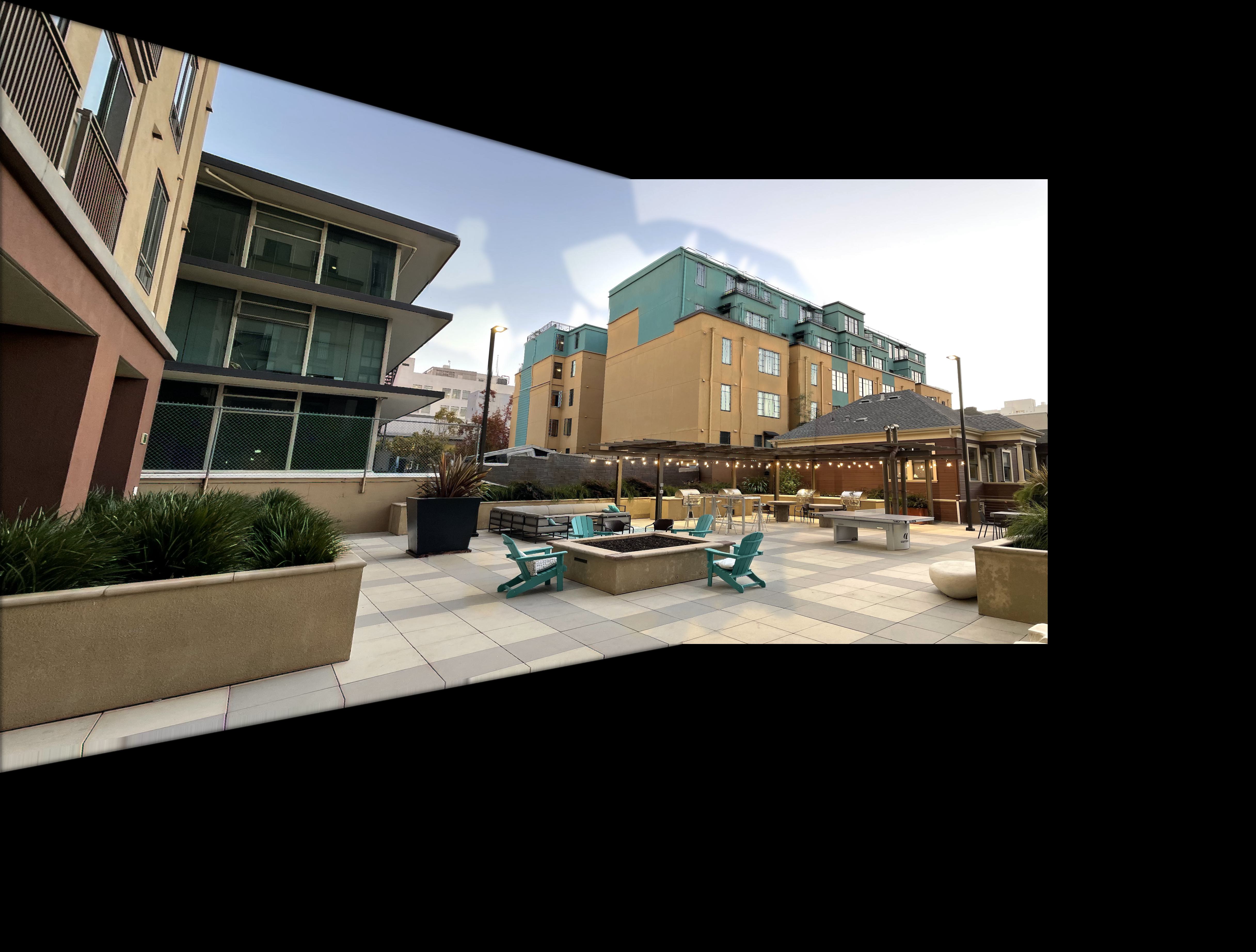
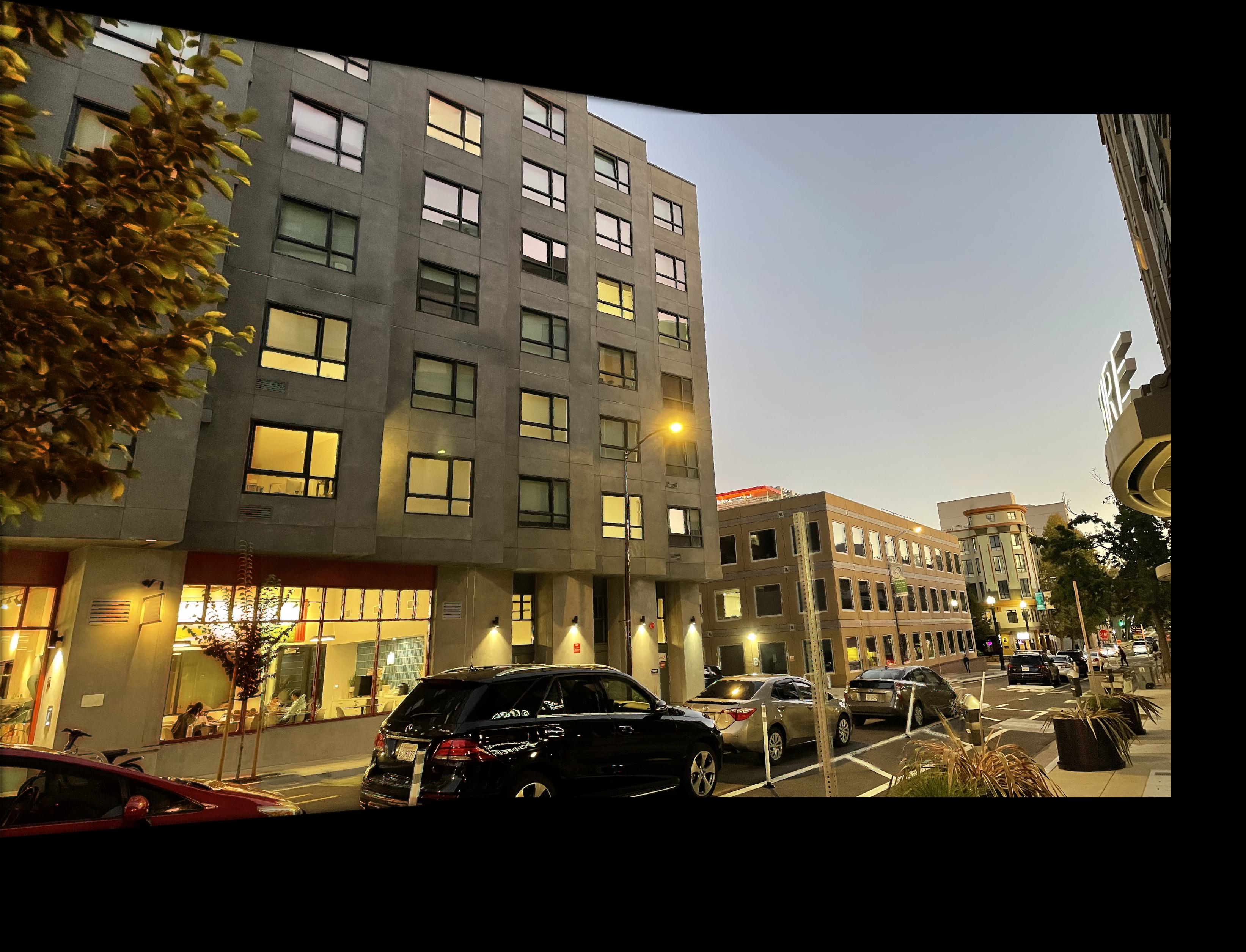
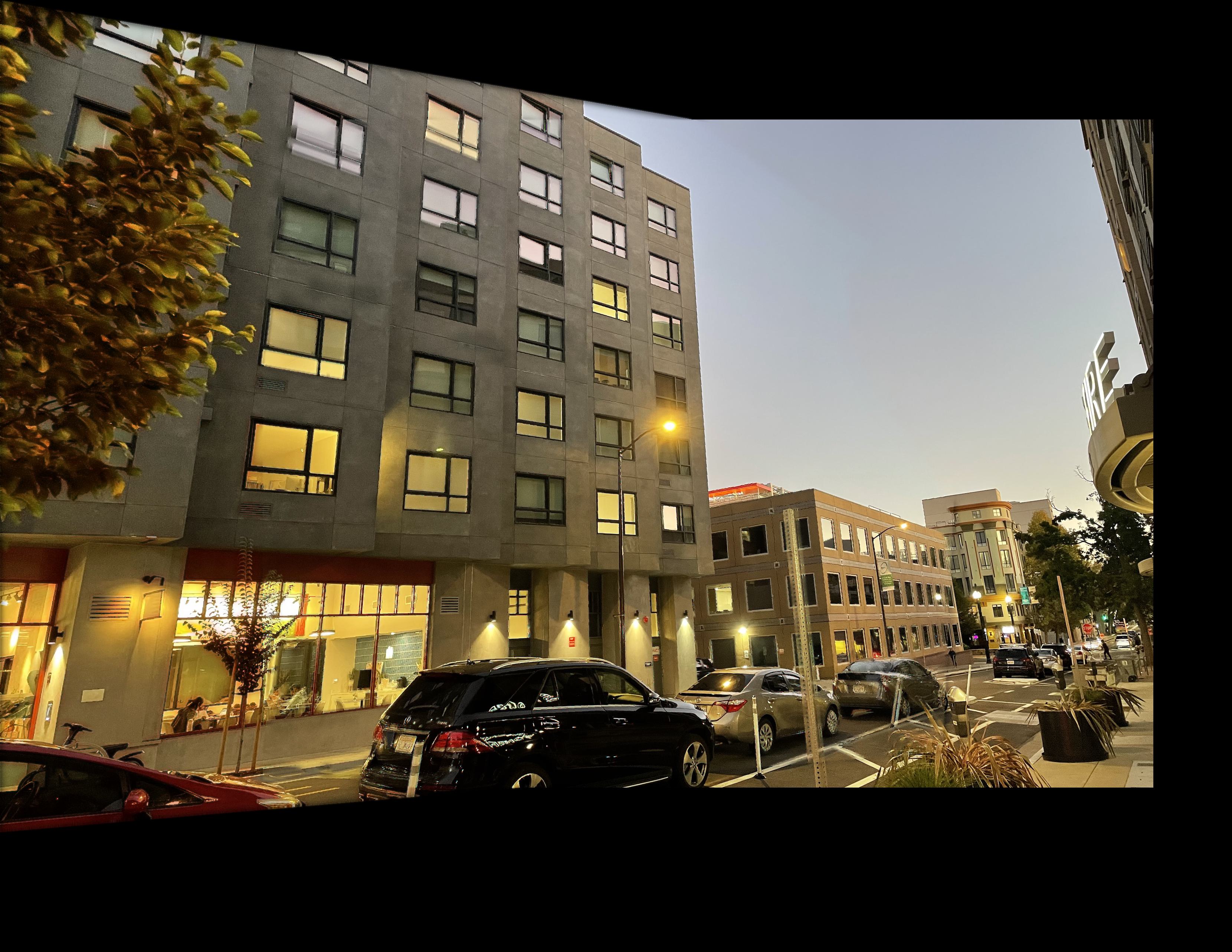
This part uses the robust homography H calculated by the method described in Part 4 to generate a complete mosaic. The results are below:

Example 1:

Example 2:

Example 3:

Conclusion

The coolest part of this project was the automatic generation of mosaics given any two images with the same center of projection.