Goal

The goal of this assignment is to experiment with diffusion models, from implementation to testing out various techniques.

Section A

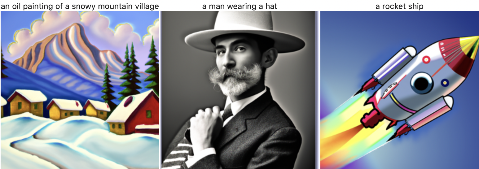
In this section, I was tasked with playing around with a pre-trained diffusion model. To start off, I displayed random model output for three pre-computed text embeddings. I generated two sets of images, the first one with 20 inference steps, and the second one with 30 inference steps.

Set 1:

Set 2:

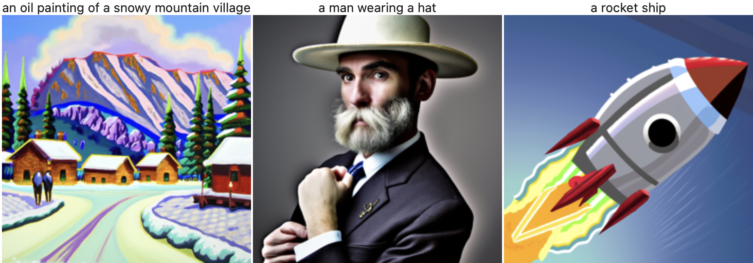
Both sets of images appear to be quite high quality, albeit a bit cartoonish for the rocket ship generated images. It is intriguing that the same pose was captured in both images of “a man wearing a hat,” although the color filter was different between the two.

Note: For all random operations in Section A, I used a seed of 108.

Part 1

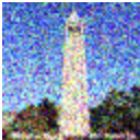
In this part, I implemented code to add random, normally distributed noise to an image. This code would be useful for later parts, where I add noise to an image, and the model should learn how to denoise an image.

Here, t stands for the time step. Higher t values indicate more noise is added to the image.

Before using the diffusion model to denoise an image, I tried using a simple gaussian blur technique to smooth out the image (take away high frequencies present in the image):

As seen above, this method did not work well, hence the need for diffusion models.

The first method I tested out with the pre-trained diffusion model was one-step denoising. Here, I passed in x_t (the noisy image) and t (the “time step”) to the UNet, in an attempt to denoise the image in one pass. The results are as follows:

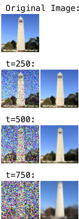
Although this one-step method fared better than the naïve Gaussian blur approach, it still did not produce desirable output. Particularly, for higher values of t, the model output gets progressively further from the ground truth.

One method to solve this issue is iteratively. In other words, the ground truth estimate can be updated over several time steps, starting from mostly noise (t = 990) to (ideally) no noise (t = 0). The results from this method are shown below:

Given that we can use the diffusion model to iteratively denoise an image, we can iteratively denoise random, normally distributed noise. Starting from pure noise allows us to generate images from scratch, with no ground truth to go off of. I generated a sample of 5 images, all with the text prompt “a high quality photo”:

Evidently, these images aren’t very coherent. To fix this, I implemented a process called Classifier Free Guidance (CFG). Here, I used the text prompt “a high quality photo” as my conditional prompt, and the null prompt “” as my unconditional prompt. I generated 5 new images using this technique with the guidance scale set to 7:

Evidently, these images are much higher quality than those produced without CFG.

Another technique is SDEdit, where the original image is perturbed with noise. Then, over a series of “edits,” or iterative denoising patterns, the original image is recovered. I tested out this process with varying starting indices (lower starting index means that the starting image is closer to pure noise).

This process worked decently well and eventually recovered something close to the original image:

I tested out this SDEdit method for a few more sets of images. The first one is obtained from the web, and the other two were hand drawn.

Set 1 (web image):

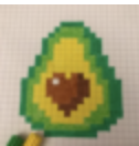
Set 2 (hand drawn):

Set 3 (hand drawn):

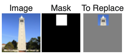
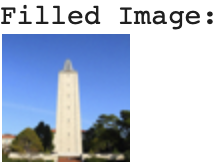
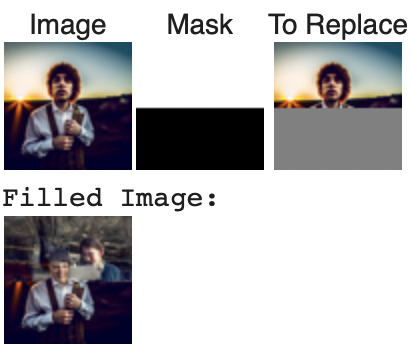
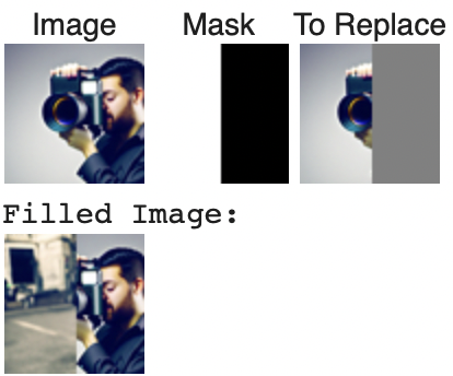
I also used the diffusion model to perform inpainting, where I filled in an image that had some portions removed based on the test image:

Set 1:

Set 2 (custom):

Set 3(custom):

I also did conditional image-to-image translation, where I started with a prompt of “a rocket ship” and ended with the original image (the Campanile).

I implemented visual anagrams, where I used one prompt to denoise one orientation of the image, and used another prompt to denoise another orientation of the image. The result is an image that looks like the first prompt when facing up, and looks like the other prompt when facing the other way:

Set 1:

Set 2:

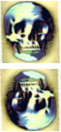
Set 3:

Finally, I generated hybrid images (something that changes in appearance based on distance to image). I considered the high frequency noise of one prompt, and the low frequency noise of the other prompt. The results are as follows:

Set 1:

Set 2:

Set 3:

Section B

In this section, I was tasked with training a diffusion model from scratch.

Part 1

In this first part, I used a UNet to train a denoiser network on the MNIST dataset. I optimized over the denoising problem, where I minimize the L2 loss between the denoised image and the ground truth image. I visualized the denoising process for various noisy images:

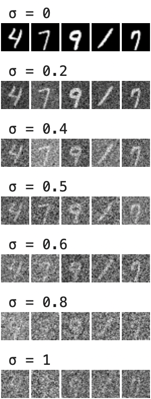
Here, higher sigma values correspond to higher levels of noise being added to the original image. The noise, as in Section A, is normally distributed.

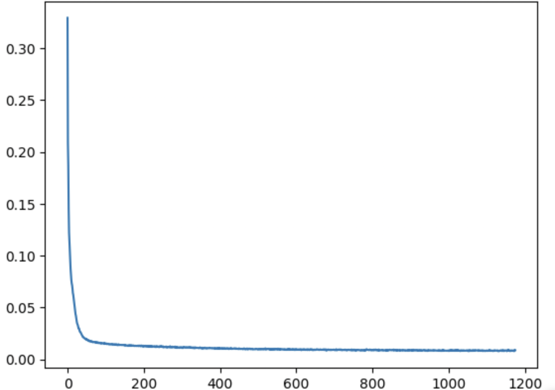
Next, I trained the UNet denoiser network to denoise images with sigma=0.5. The training cycle involved a batch size of 256, with 5 total epochs. I used a UNet architecture with hidden dimension D = 128, and an Adam optimizer with a learning rate of 1e-04. Below is a plot of my training losses over each batch:

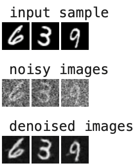
Here are results for denoising after 1 epoch of training:

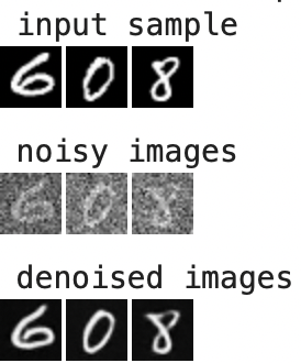
Below are results for denoising after 5 epochs of training:

I also tested the model with out-of-distribution images (passing in noisy images with sigma values not necessarily equal to 0.5):

Part 2

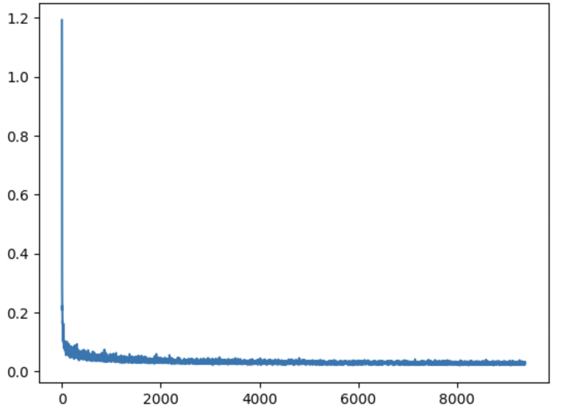
In this part, I trained a diffusion model to iteratively denoise images. Specifically, I added time-conditioning to the UNet. Therefore, the model could predict the denoised image given the noisy image and the current time step t. For this training cycle, I used a batch size of 128, with 20 total epochs. I used a UNet architecture with hidden dimension D = 64, and an Adam optimizer with learning rate 1e-03. I also added an exponential learning rate decay scheduler. Below is a plot of my training losses over each batch:

Part 3

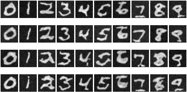
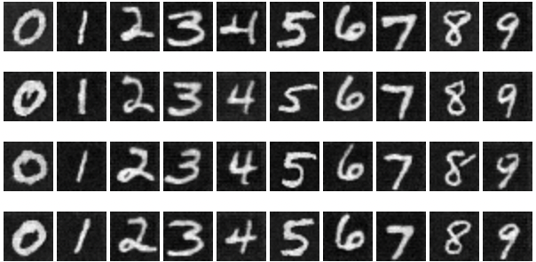
Below are my denoising results for select epochs during the training cycle:

Part 4

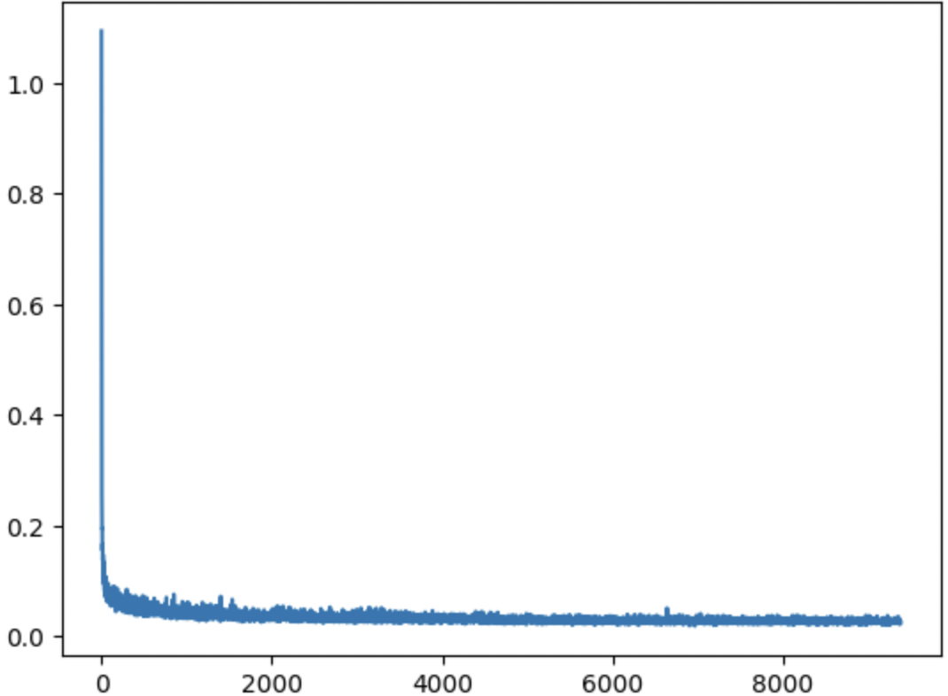
In this part, I trained a diffusion model to iteratively denoise images. Here, I added class-conditioning to the UNet in addition to time-conditioning. Therefore, the model could predict the denoised image based on the class (numeral) of the image. For this training cycle, I used a batch size of 128, with 20 total epochs. I used a UNet architecture with hidden dimension D = 64, and an Adam optimizer with learning rate 1e-03. I also added an exponential learning rate decay scheduler. Below is a plot of my training losses over each batch:

Part 5

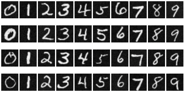
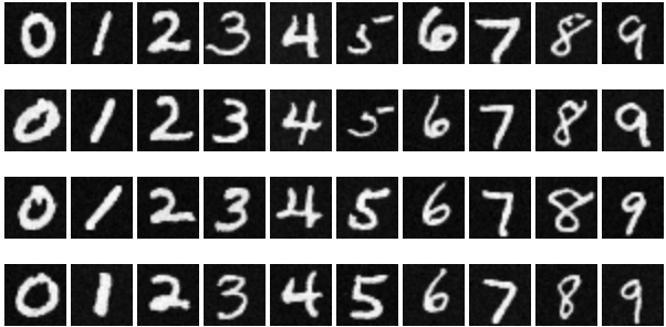
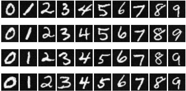
For this part, I sampled generated images based on all classes with classifier free guidance (CFG). Below are my denoising results for select epochs during the training cycle: